Hierarchical forecasting of hospital admissions- EDA part 2
Introduction
The aim of this series of blog is to predict monthly admissions to Singapore public acute adult hospitals. The dataset starts from Jan 2016 and ends in Feb 2021.
library(tidyverse)
library(timetk)
library(fpp3)

# cleaned up dataset downloaded from  my github. Clean up of OG dataset done in 1st post
raw<- read_csv("https://raw.githubusercontent.com/notast/hierarchical-forecasting/main/stat_sg_CLEAN.csv")

# dataset w national total; recalculate total hospital admissions
df<-raw %>% group_by(Date) %>% summarise(Admission=sum(Admission, na.rm = T)) %>% mutate(Cluster= "National", Hospital= "National") %>% bind_rows(raw)
EDA for trend, seasonality and anomalies were explored in the last post. This post will complete EDA with lags and correlation of features of the time series.
1. Lags
Lags can be used to screen for seasonality. The values of lags can be used to calculate auto-correlation (ACF) and partial autocorrelation (PACF) There are two approaches for using lags for forecasting:
- Short lags (lag length < forecast horizon)
When the lag length (e.g. 1 month) is less than the forecast horizon (e.g. 3 months), missing values are generated in future data which may pose a problem for some forecasting models.
df %>%  group_by(Hospital) %>%
  future_frame(.date_var= Date, .length_out = "3 months", .bind_data = T) %>% ungroup() %>%
  mutate(Lag1month= lag_vec(Admission, lag=1)) %>%
  tail()
## # A tibble: 6 x 5
## Hospital Date Admission Cluster Lag1month
## <chr> <date> <dbl> <chr> <dbl>
## 1 TTSH 2020-12-01 4719 NHG 4210
## 2 TTSH 2021-01-01 4502 NHG 4719
## 3 TTSH 2021-02-01 4235 NHG 4502
## 4 TTSH 2021-03-01 NA <NA> 4235
## 5 TTSH 2021-04-01 NA <NA> NA
## 6 TTSH 2021-05-01 NA <NA> NARecursive predictions are iterated to artificially generate lags (e.g. lag of 1 month again and again). Recursive prediction is used in ARIMA.
- Long term lags (lag length >= forecast horizon)
Long-term lags can be used to create lagged rolling features, which have proven predictive properties in the M5 competition. A disadvantage of using long term lags is the absent of short term lags which may have predictive properties.
1.1 Auto-correlation (ACF)
- ACF measures the linear relationship between lagged values of a time series. It measures how much the most recent value of the series is correlated with past values of the series, there is a tendency for values in a time series to be correlated with past observations in that time series.
- [If the time series has a trend, the ACF for small lags tend to be positive and large because observations nearby in time are also nearby in size.
- If the time series has seasonality, the ACF will have spikes. The autocorrelations will be larger at multiples of seasonal frequency than other lags.]( https://otexts.com/fpp3/acf.html) e.g. for a daily dataset, if there are a spikes at day 7 and day 14, there is weekly seasonality. Nonetheless, if the spike at day 14 is larger than day 7, something is happening at the week 2 interval.
- ACF can also provide candidate periods for Fourier terms. A regression model containing Fourier terms (aka harmonic regression) is better for time series with longer seasonal periods (even seasonal ARIMA and seasonal ETS have ceiling seasonality periods). The longer seasonal pattern is modelled using Fourier terms while the short term dynamics can be modelled with ARIMA or ETS.
1.2 Partial Autocorrelation (PACF)
PACF measures the linear relationship between the correlations of the residuals (while ACF measures the linear relationship between lagged values). Using the correlation of residuals, PACF removes the dependence of lags on other lags. e.g. it looks at the direct effect between Jan and Mar and omits indirect effect between Jan to Feb and Feb to Mar.
ACF tells us which lags are important while PACF tells us which lags are different and have functional implications.
- Based on the seasonality year strength values, CGH has the highest yearly seasonality. Spikes can be seen for CGH at lag 12 and 24 for CGH’s ACF plot and spikes can be seen at lag 12 for CGH’s PACF plot (CGH is plot 2).
- AH and SKH are hospitals with the lowest seasonality year strength values. Their ACF and PACF plots have no spikes (AH is plot 1 and SKH is plot 6).
- The time series are unlikely white noises as one or more large spikes are outside these bound
plt_acf<-df %>% nest(-Hospital)%>%
  mutate(p= map2(.x=data, .y=Hospital, ~
                plot_acf_diagnostics(
                .data=.x,
                .date_var = Date, .value = Admission,
                .show_white_noise_bars = TRUE,.interactive = F, .title=.y)))
## Warning: All elements of `...` must be named.
## Did you want `data = c(Date, Admission, Cluster)`?## Max lag exceeds data available. Using max lag: 61
## Max lag exceeds data available. Using max lag: 61
## Max lag exceeds data available. Using max lag: 61
## Max lag exceeds data available. Using max lag: 61
## Max lag exceeds data available. Using max lag: 61
## Max lag exceeds data available. Using max lag: 61
## Max lag exceeds data available. Using max lag: 61
## Max lag exceeds data available. Using max lag: 61
## Max lag exceeds data available. Using max lag: 61plt_acf$p## [[1]]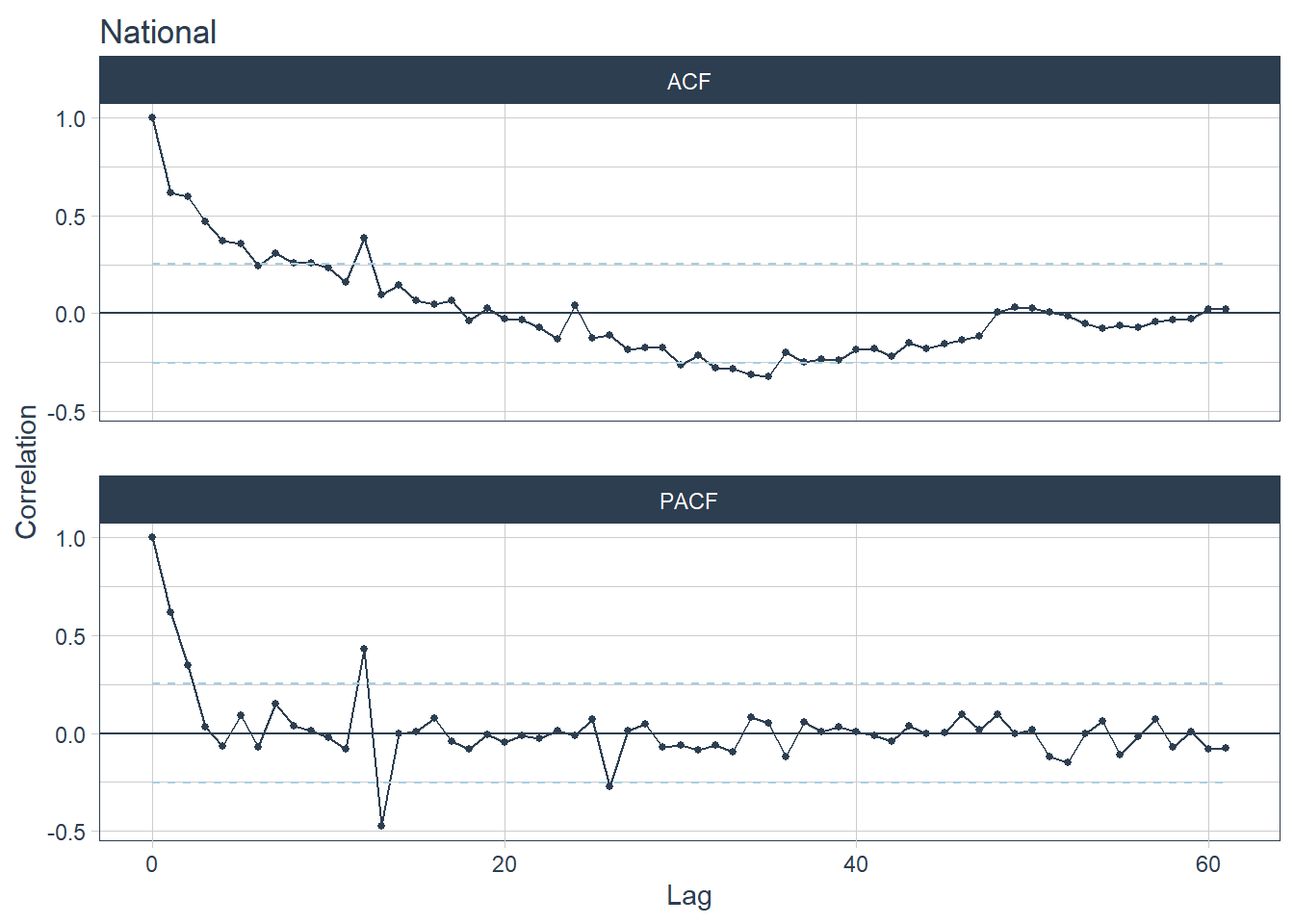
##
## [[2]]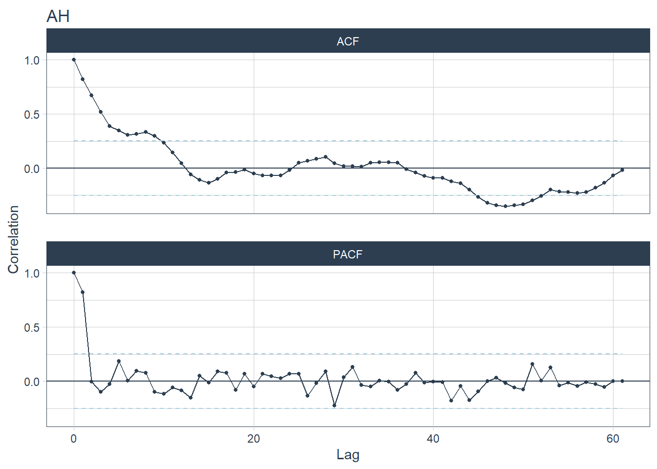
##
## [[3]]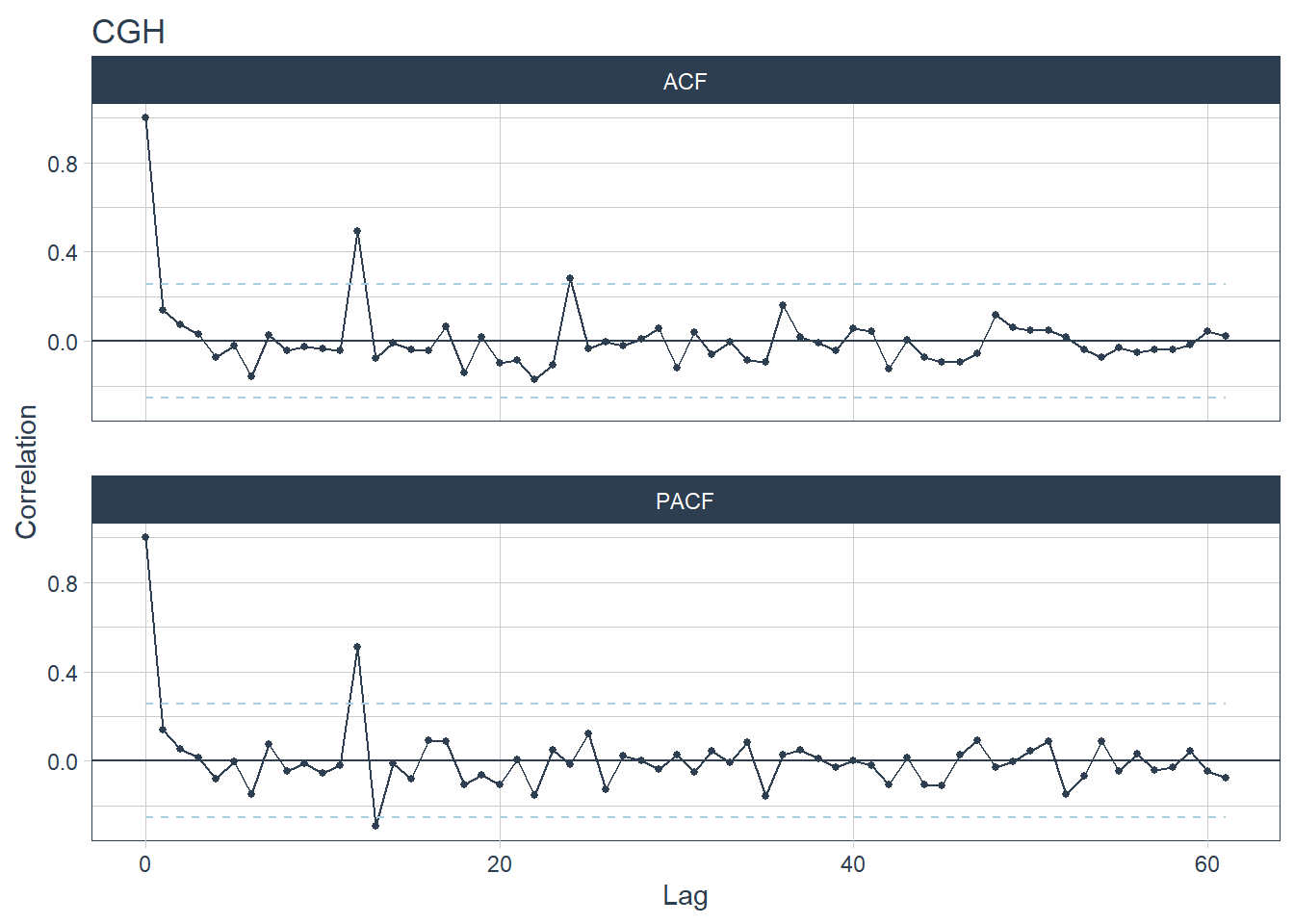
##
## [[4]]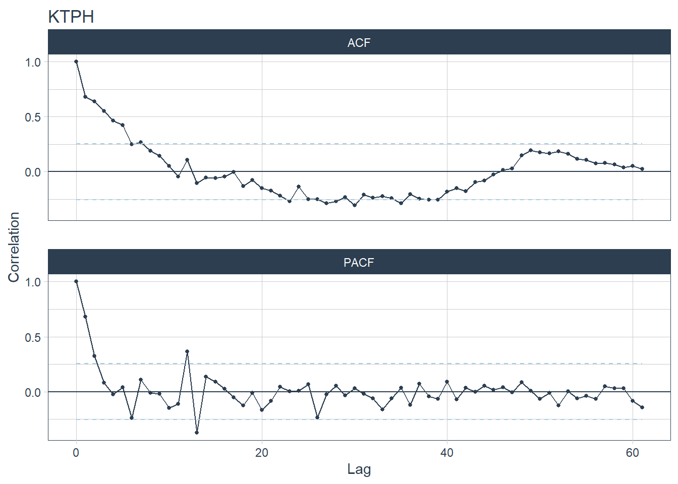
##
## [[5]]
##
## [[6]]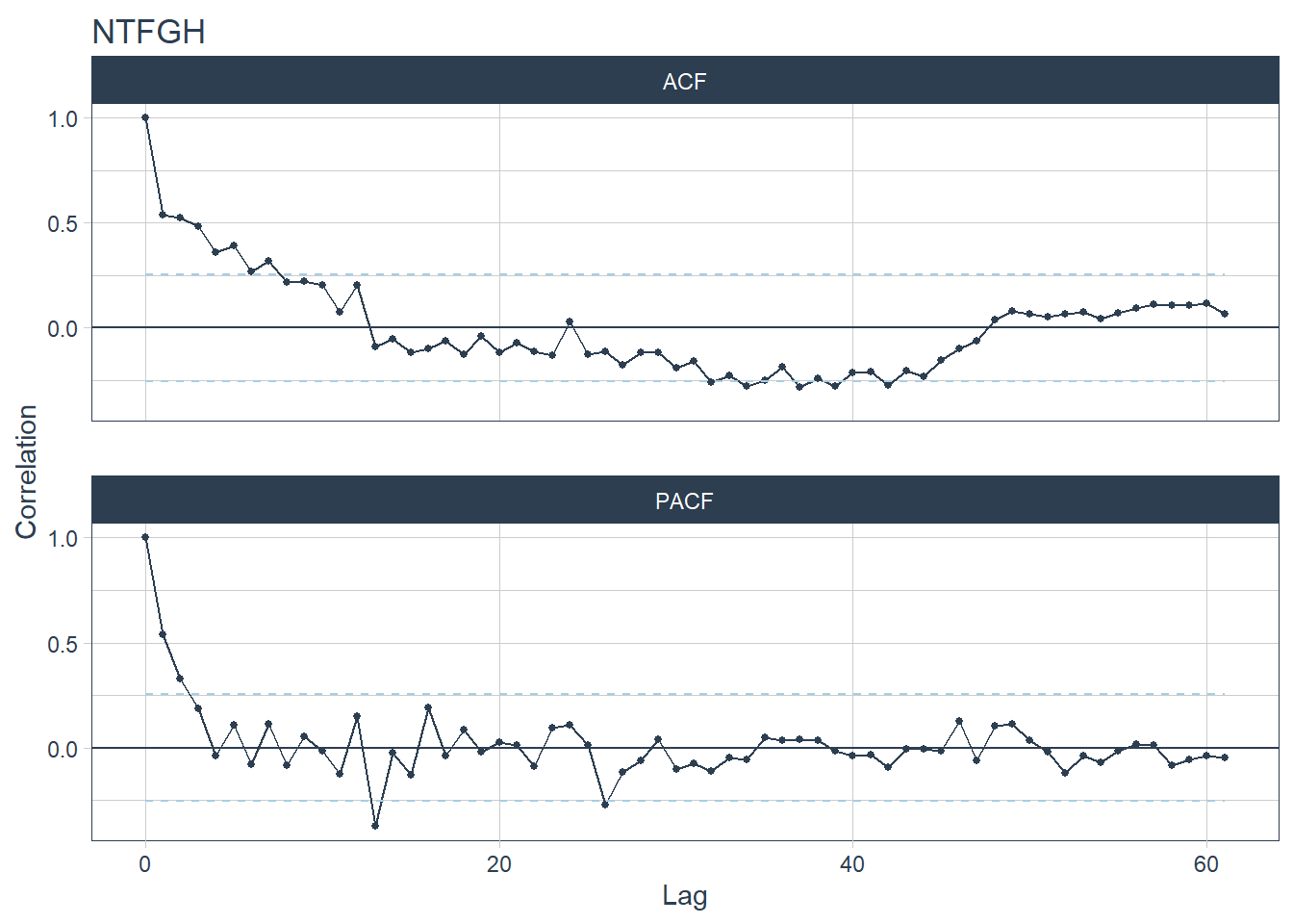
##
## [[7]]
## Warning: Removed 30 row(s) containing missing values (geom_path).## Warning: Removed 60 rows containing missing values (geom_point).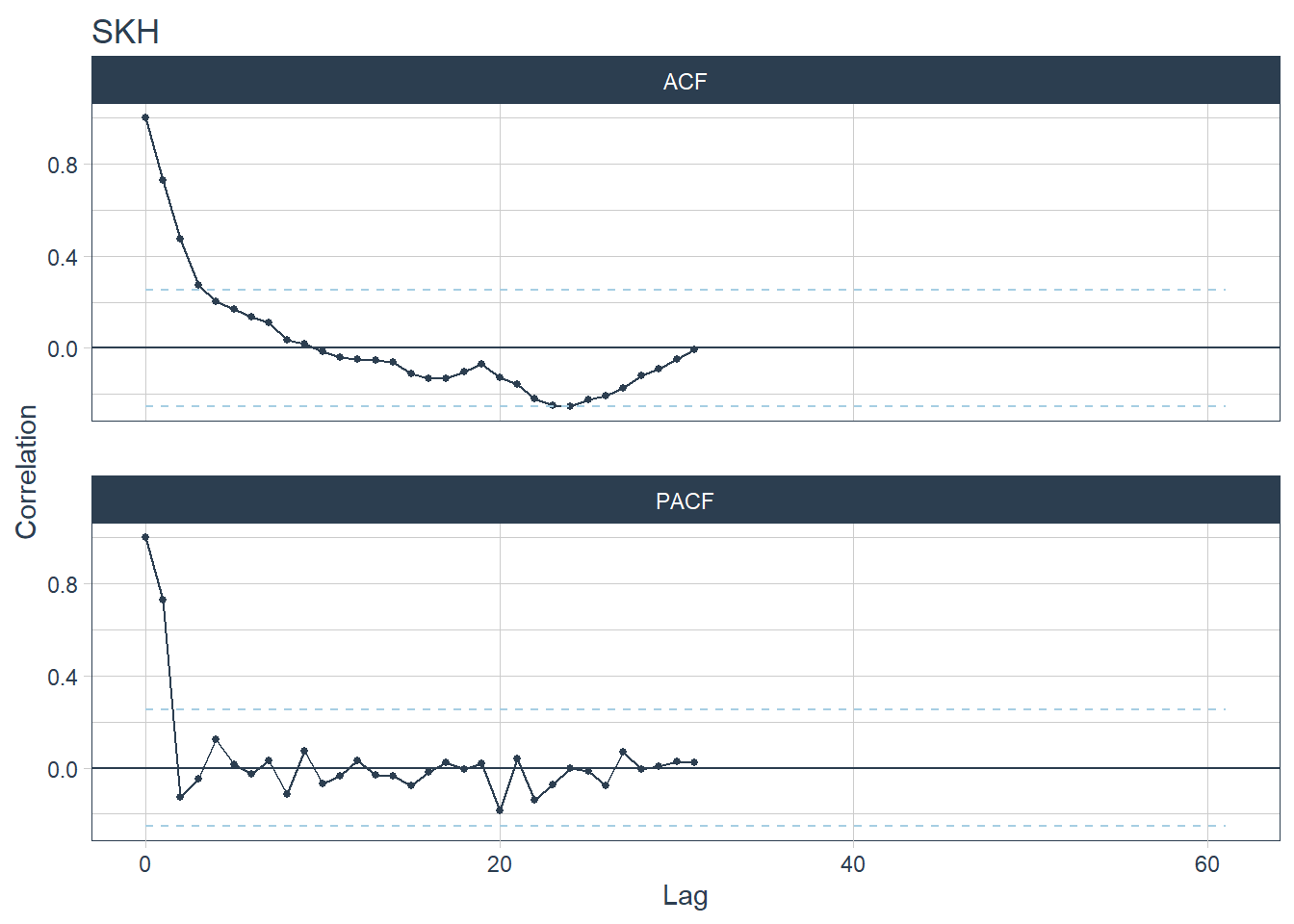
##
## [[8]]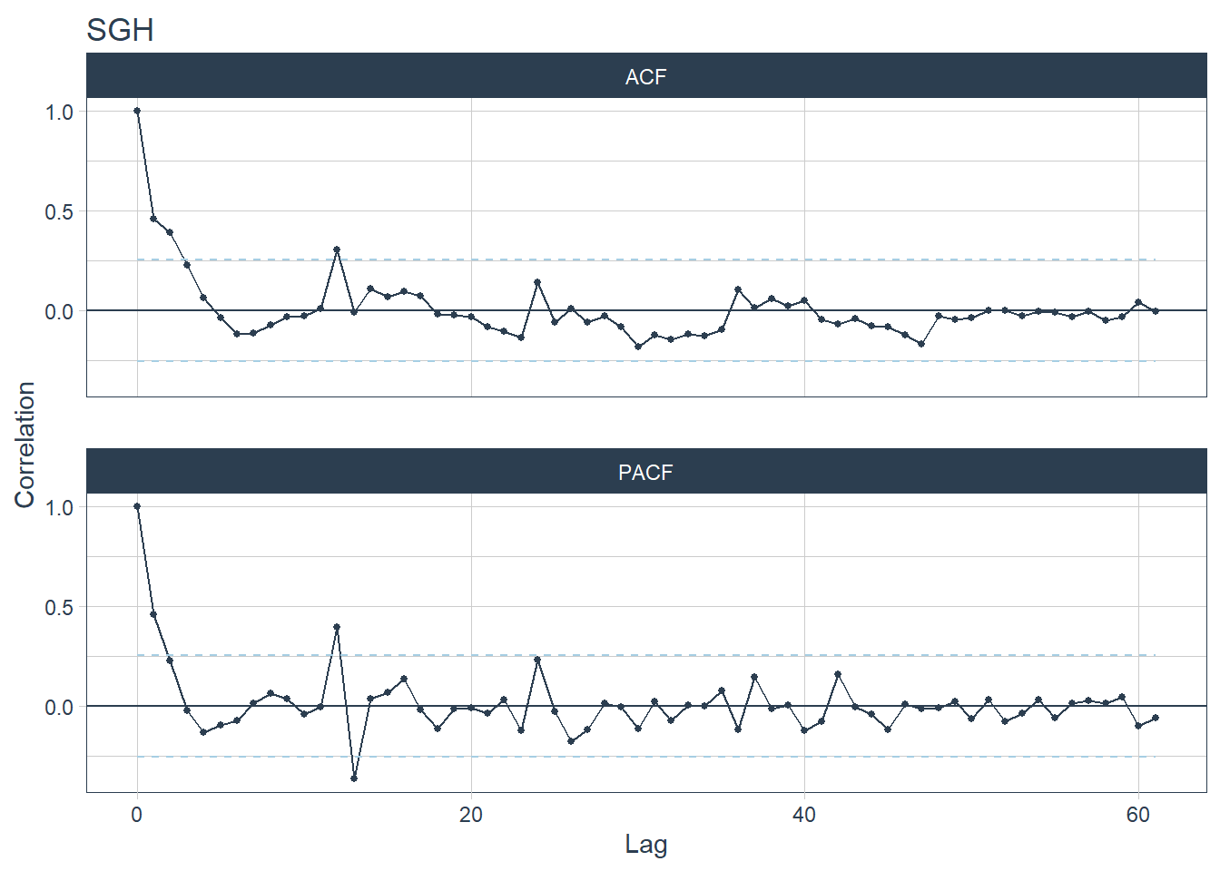
##
## [[9]]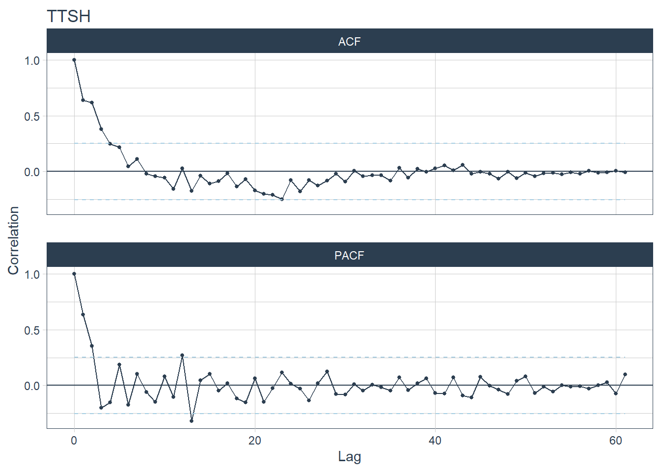
2. Correlation of features
Features and statistical values can be extracted from a time series. The fpp3 meta-package has a library feasts which provide provides up to 48 features. The features are tagged to 22 relevant concepts. 48 features is a relatively large number of variables to analyze, the correlation can help determine the associative relationship between the features.
The desired features are established with fabletools::feature_set and the features are extracted with fabeltools::features.
Every country has an organisation order to its public hospitals. In Singapore, there are 3 levels:
|– Cluster level (Clusters are a network of hospitals based based on geographical regions. There are 3 health clusters in Singapore.)
|– Hospital level (There are 8 public acute adult hospitals.)
Features for each hierarchical level will be created.
feat_hos<- df%>%
  filter(Hospital!= "National") %>%
  mutate(Date= yearmonth(as.character(Date))) %>%
  as_tsibble(key= Hospital , index= Date) %>%
  features(Admission, feature_set(pkgs="feasts")) %>%
  mutate(Level="Hospital_id") %>% rename(Name=Hospital)
## Warning: `n_flat_spots()` was deprecated in feasts 0.1.5.
## Please use `longest_flat_spot()` instead.## Warning: 1 error encountered for feature 3
## [1] missing values in object## Warning: 1 error encountered for feature 4
## [1] missing value where TRUE/FALSE needed## Warning: 1 error encountered for feature 5
## [1] missing value where TRUE/FALSE needed## Warning: 1 error encountered for feature 9
## [1] series is not periodic or has less than two periods## Warning: 1 error encountered for feature 20
## [1] invalid time series parameters specifiedfeat_clu<- df%>%
filter(Cluster!= "National") %>%
group_by(Cluster, Date) %>% summarise(Admission= sum(Admission, na.rm = T), .groups= "drop") %>%
mutate(Date= yearmonth(as.character(Date))) %>%
as_tsibble(key= Cluster , index= Date) %>%
features(Admission, feature_set(pkgs="feasts")) %>%
mutate(Level="Cluster_id") %>% rename(Name=Cluster)
feat_sg<- df %>% filter(Hospital=="National") %>%
mutate(Date= yearmonth(as.character(Date))) %>%
as_tsibble(key= Hospital , index= Date) %>%
features(Admission, feature_set(pkgs="feasts")) %>%
mutate(Level="National_id") %>% rename(Name=Hospital)
feat_all<- bind_rows(feat_hos, feat_clu, feat_sg)
glimpse(feat_all)## Rows: 12
## Columns: 50
## $ Name <chr> "AH", "CGH", "KTPH", "NTFGH", "NUH", "SGH", "SK~
## $ trend_strength <dbl> 0.8008467, 0.2753427, 0.7806859, 0.8074394, 0.7~
## $ seasonal_strength_year <dbl> 0.2054133, 0.6550050, 0.4371513, 0.5688091, 0.5~
## $ seasonal_peak_year <dbl> 7, 0, 0, 10, 10, 7, 10, 0, 0, 10, 10, 10
## $ seasonal_trough_year <dbl> 2, 2, 2, 2, 2, 2, 8, 2, 2, 2, 2, 2
## $ spikiness <dbl> 34308.47, 157238.54, 191874.46, 56234.36, 17971~
## $ linearity <dbl> 1131.4782, 347.8845, -512.1808, -759.2038, 753.~
## $ curvature <dbl> -97.4100, -313.7077, -1564.4875, -1325.6676, -2~
## $ stl_e_acf1 <dbl> 0.49046893, 0.17755315, 0.48299062, -0.01179575~
## $ stl_e_acf10 <dbl> 0.8845025, 0.3302167, 0.6178947, 0.1922015, 0.7~
## $ acf1 <dbl> 0.8206216, 0.1402620, 0.6816803, 0.5401742, 0.6~
## $ acf10 <dbl> 2.11098809, 0.06089474, 1.76735644, 1.39798436,~
## $ diff1_acf1 <dbl> -0.1443261, -0.4596242, -0.4699489, -0.5438977,~
## $ diff1_acf10 <dbl> 0.1936206, 0.2893855, 0.4387209, 0.5788380, 0.4~
## $ diff2_acf1 <dbl> -0.5765913, -0.6587037, -0.6950116, -0.7213507,~
## $ diff2_acf10 <dbl> 0.5990664, 0.6023470, 0.8644087, 0.9993514, 0.9~
## $ season_acf1 <dbl> 0.04584300, 0.49355004, 0.10840987, 0.20553676,~
## $ pacf5 <dbl> 0.7185930, 0.0294867, 0.5769965, 0.4474341, 0.5~
## $ diff1_pacf5 <dbl> 0.2053477, 0.7647219, 0.6325854, 0.6161773, 0.6~
## $ diff2_pacf5 <dbl> 0.6957611, 1.1845925, 1.2335587, 1.3390279, 1.2~
## $ season_pacf <dbl> -0.0848245, 0.5090732, 0.3632837, 0.1520572, 0.~
## $ zero_run_mean <dbl> 0, 0, 0, 0, 0, 0, NA, 0, 0, 0, 0, 0
## $ nonzero_squared_cv <dbl> 0.131243894, 0.002854840, 0.007221997, 0.006827~
## $ zero_start_prop <dbl> 0, 0, 0, 0, 0, 0, NA, 0, 0, 0, 0, 0
## $ zero_end_prop <dbl> 0, 0, 0, 0, 0, 0, NA, 0, 0, 0, 0, 0
## $ lambda_guerrero <dbl> 1.2755867, 0.4304620, 1.9999268, 1.1297130, 1.9~
## $ kpss_stat <dbl> 1.0798491, 0.2729302, 0.4187294, 0.6144483, 0.3~
## $ kpss_pvalue <dbl> 0.01000000, 0.10000000, 0.06908217, 0.02132288,~
## $ pp_stat <dbl> -2.764480, -6.575707, -3.028578, -3.247063, -3.~
## $ pp_pvalue <dbl> 0.07280602, 0.01000000, 0.04242816, 0.02856648,~
## $ ndiffs <int> 1, 0, 0, 1, 0, 0, 2, 0, 0, 0, 1, 1
## $ nsdiffs <int> 0, 1, 0, 0, 0, 0, NA, 0, 0, 0, 0, 0
## $ bp_stat <dbl> 41.752026, 1.219753, 28.810659, 18.090865, 26.9~
## $ bp_pvalue <dbl> 1.036148e-10, 2.694091e-01, 7.981068e-08, 2.106~
## $ lb_stat <dbl> 43.805404, 1.279741, 30.227576, 18.980579, 28.2~
## $ lb_pvalue <dbl> 3.627021e-11, 2.579472e-01, 3.842076e-08, 1.320~
## $ var_tiled_var <dbl> 0.019075484, 0.390044129, 0.029382931, 0.007222~
## $ var_tiled_mean <dbl> 0.7902109, 0.1644186, 0.7186914, 1.5074989, 0.7~
## $ shift_level_max <dbl> 290.2500, 222.6667, 488.4167, 406.0833, 776.583~
## $ shift_level_index <dbl> 14, 3, 50, 7, 50, 50, 33, 50, 50, 14, 34, 50
## $ shift_var_max <dbl> 22794.73, 66035.73, 111015.11, 42842.55, 368944~
## $ shift_var_index <dbl> 21, 44, 43, 43, 43, 43, 38, 43, 43, 43, 26, 43
## $ shift_kl_max <dbl> 3.1278495, 0.9981751, 1.7897819, 2.0810018, 1.2~
## $ shift_kl_index <dbl> 14, 2, 49, 2, 49, 2, 33, 49, 49, 14, 33, 49
## $ spectral_entropy <dbl> 0.6737795, 0.8638561, 0.7099517, 0.6770887, 0.7~
## $ n_crossing_points <int> 15, 26, 14, 22, 12, 22, 8, 19, 18, 18, 1, 20
## $ longest_flat_spot <int> 4, 4, 3, 3, 4, 7, 7, 4, 4, 4, 4, 4
## $ coef_hurst <dbl> 0.9874871, 0.6018881, 0.9615349, 0.9336814, 0.9~
## $ stat_arch_lm <dbl> 0.3423610, 0.3639838, 0.3467997, 0.3723909, 0.2~
## $ Level <chr> "Hospital_id", "Hospital_id", "Hospital_id", "H~Missing values need to be dropped before the correlation can be calculated. 11/48 features have missing values
(feat_ms<-feat_all %>% select_if(function(x) any(is.na(x))) %>% colnames())## [1] "pacf5" "diff1_pacf5" "diff2_pacf5"
## [4] "season_pacf" "zero_run_mean" "nonzero_squared_cv"
## [7] "zero_start_prop" "zero_end_prop" "lambda_guerrero"
## [10] "nsdiffs" "coef_hurst"The missing values are from SKH likely due to nil admissions before it was open in Jul 2018. We are unable to drop observations with NA values as that will mean removing the SKH so we removed variables with missing values. The time series features is reduced from 48 to 37.
feat_all %>% filter_all(any_vars(is.na(.)))## # A tibble: 1 x 50
## Name trend_strength seasonal_strength_y~ seasonal_peak_ye~ seasonal_trough_y~
## <chr> <dbl> <dbl> <dbl> <dbl>
## 1 SKH 0.838 0.284 10 8
## # ... with 45 more variables: spikiness <dbl>, linearity <dbl>,
## # curvature <dbl>, stl_e_acf1 <dbl>, stl_e_acf10 <dbl>, acf1 <dbl>,
## # acf10 <dbl>, diff1_acf1 <dbl>, diff1_acf10 <dbl>, diff2_acf1 <dbl>,
## # diff2_acf10 <dbl>, season_acf1 <dbl>, pacf5 <dbl>, diff1_pacf5 <dbl>,
## # diff2_pacf5 <dbl>, season_pacf <dbl>, zero_run_mean <dbl>,
## # nonzero_squared_cv <dbl>, zero_start_prop <dbl>, zero_end_prop <dbl>,
## # lambda_guerrero <dbl>, kpss_stat <dbl>, kpss_pvalue <dbl>, pp_stat <dbl>,
## # pp_pvalue <dbl>, ndiffs <int>, nsdiffs <int>, bp_stat <dbl>,
## # bp_pvalue <dbl>, lb_stat <dbl>, lb_pvalue <dbl>, var_tiled_var <dbl>,
## # var_tiled_mean <dbl>, shift_level_max <dbl>, shift_level_index <dbl>,
## # shift_var_max <dbl>, shift_var_index <dbl>, shift_kl_max <dbl>,
## # shift_kl_index <dbl>, spectral_entropy <dbl>, n_crossing_points <int>,
## # longest_flat_spot <int>, coef_hurst <dbl>, stat_arch_lm <dbl>, Level <chr># drop na columns
feat_all<- feat_all %>% select(-all_of(feat_ms))The correlation for each level is visualized below.
Hospital level
fun_corrplt<- function(L,T){
  feat_all %>%
  filter(Level==L) %>%
  #  cor only takes numeric values
  select(-c(Level, Name)) %>% cor() %>%
  corrplot::corrplot(type="lower", order="hclust", tl.col="black", tl.srt=80, tl.cex=0.65, title = T)}

fun_corrplt("Hospital_id", "Hospital level")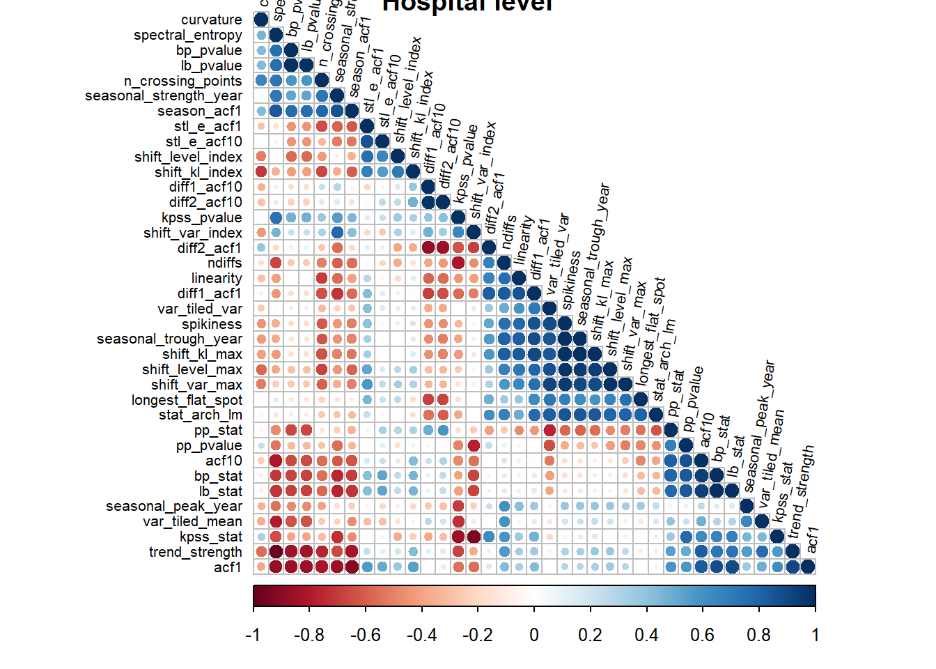
Cluster level
fun_corrplt("Cluster_id", "Cluster level")## Warning in cor(.): the standard deviation is zero## Error in hclust(as.dist(1 - corr), method = hclust.method): NA/NaN/Inf in foreign function call (arg 10)National level
fun_corrplt("National_id", "National level")## Warning in min(corr, na.rm = TRUE): no non-missing arguments to min; returning
## Inf## Warning in max(corr, na.rm = TRUE): no non-missing arguments to max; returning
## -Inf## Error in hclust(as.dist(1 - corr), method = hclust.method): NA/NaN/Inf in foreign function call (arg 10)All levels
Correlation at all levels was collectively calculated as admissions at a superordinate levels would have some correlation with admissions at the subordinate level.
fun_corrplt(c("Hospital_id", "Cluster_id", "National_id"), "All levels")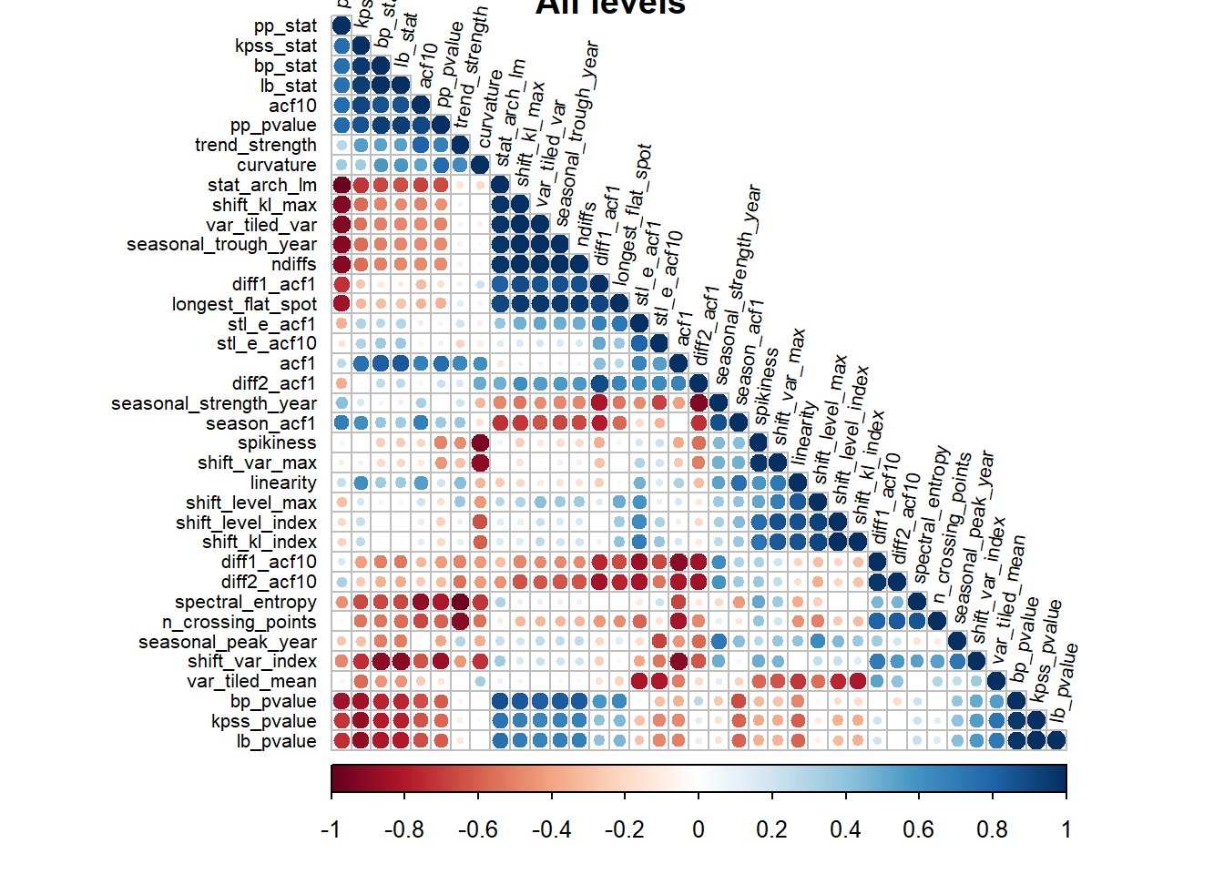
Correlation findings
- Correlation could not be calculated at cluster level and national level, likely due to limited to observations.
- There are more features which are correlated at the collective level than at the hospital level.
- The spread in the correlations revealed the heterogenity of the features, the features identify a variety of time series traits.
2.1 PCA of features
library(recipes)

(feat_pca_rec<-feat_all %>% recipe(~.) %>%
  update_role(Name, new_role = "id") %>% update_role(Level, new_role = "id") %>%
  step_normalize(all_numeric_predictors()) %>%
  step_pca(all_numeric_predictors()))
## Data Recipe
##
## Inputs:
##
## role #variables
## id 2
## predictor 37
##
## Operations:
##
## Centering and scaling for all_numeric_predictors()
## No PCA components were extracted.feat_pca_rec %>% tidy()## # A tibble: 2 x 6
## number operation type trained skip id
## <int> <chr> <chr> <lgl> <lgl> <chr>
## 1 1 step normalize FALSE FALSE normalize_uuOrN
## 2 2 step pca FALSE FALSE pca_jfihNfeat_pca_rec %>% summary()## # A tibble: 39 x 4
## variable type role source
## <chr> <chr> <chr> <chr>
## 1 Name nominal id original
## 2 trend_strength numeric predictor original
## 3 seasonal_strength_year numeric predictor original
## 4 seasonal_peak_year numeric predictor original
## 5 seasonal_trough_year numeric predictor original
## 6 spikiness numeric predictor original
## 7 linearity numeric predictor original
## 8 curvature numeric predictor original
## 9 stl_e_acf1 numeric predictor original
## 10 stl_e_acf10 numeric predictor original
## # ... with 29 more rows2.1 Variation captured
Here we examined the variation captured for each principal component.
(feat_pca_prep<- feat_pca_rec %>% prep())## Data Recipe
##
## Inputs:
##
## role #variables
## id 2
## predictor 37
##
## Training data contained 12 data points and no missing data.
##
## Operations:
##
## Centering and scaling for trend_strength, ... [trained]
## PCA extraction with trend_strength, ... [trained]The time series features were transformed into principal components and the first 5 principal components were retained by default for step_pca
feat_pca_prep %>% summary()## # A tibble: 7 x 4
## variable type role source
## <chr> <chr> <chr> <chr>
## 1 Name nominal id original
## 2 Level nominal id original
## 3 PC1 numeric predictor derived
## 4 PC2 numeric predictor derived
## 5 PC3 numeric predictor derived
## 6 PC4 numeric predictor derived
## 7 PC5 numeric predictor derivedfeat_pca_prep %>% tidy()## # A tibble: 2 x 6
## number operation type trained skip id
## <int> <chr> <chr> <lgl> <lgl> <chr>
## 1 1 step normalize TRUE FALSE normalize_uuOrN
## 2 2 step pca TRUE FALSE pca_jfihNThe value of each time series feature from each principal component was tabulated.
feat_pca_PC<-feat_pca_prep %>% tidy(2)

feat_pca_PC
## # A tibble: 444 x 4
## terms value component id
## <chr> <dbl> <chr> <chr>
## 1 trend_strength -0.260 PC1 pca_jfihN
## 2 seasonal_strength_year 0.125 PC1 pca_jfihN
## 3 seasonal_peak_year -0.154 PC1 pca_jfihN
## 4 seasonal_trough_year -0.0732 PC1 pca_jfihN
## 5 spikiness -0.0454 PC1 pca_jfihN
## 6 linearity -0.178 PC1 pca_jfihN
## 7 curvature -0.0141 PC1 pca_jfihN
## 8 stl_e_acf1 -0.0985 PC1 pca_jfihN
## 9 stl_e_acf10 -0.0151 PC1 pca_jfihN
## 10 acf1 -0.273 PC1 pca_jfihN
## # ... with 434 more rowsThe percentage variance captured for each new principal component was plotted.
- The first 5 principal component captured 88% of the variance.
- There was no need to increase the number of components in
step_pcaas adequate variation was summarised in the first 5 components.
# https://juliasilge.com/blog/best-hip-hop/

sdev<-feat_pca_prep$steps[[2]]$res$sdev
percent_variation <- sdev^2 / sum(sdev^2)

tibble(
  component = unique(feat_pca_PC$component),
  percent_var = cumsum(percent_variation)
) %>%
  mutate(component = fct_inorder(component)) %>%
  ggplot(aes(component, percent_var)) +
  geom_col() +
  scale_y_continuous(labels = scales::percent_format()) +
  labs(x = NULL, y = "Percent variance capature by adding another PCA component")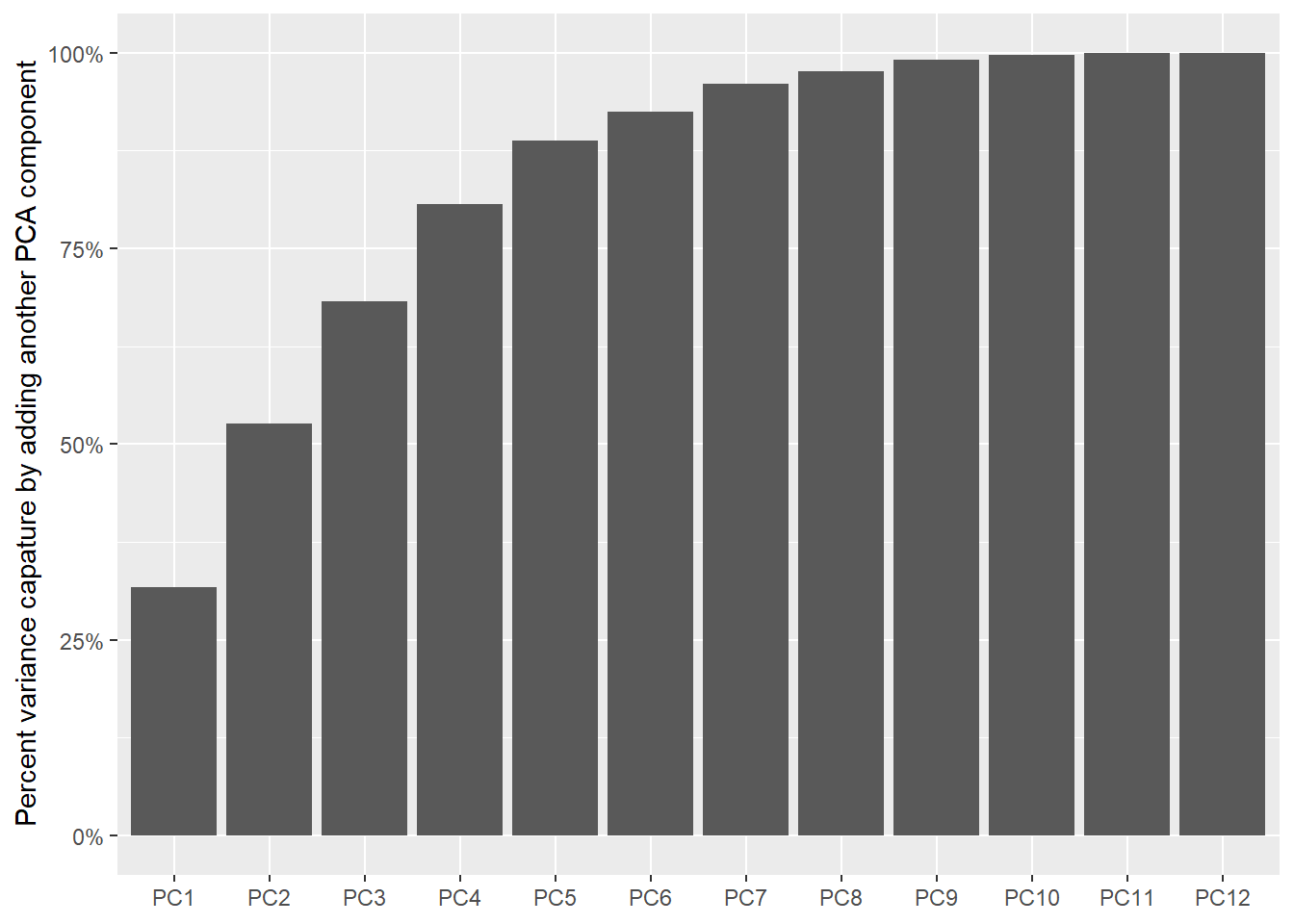
2.2 Time series features contributing to PC1
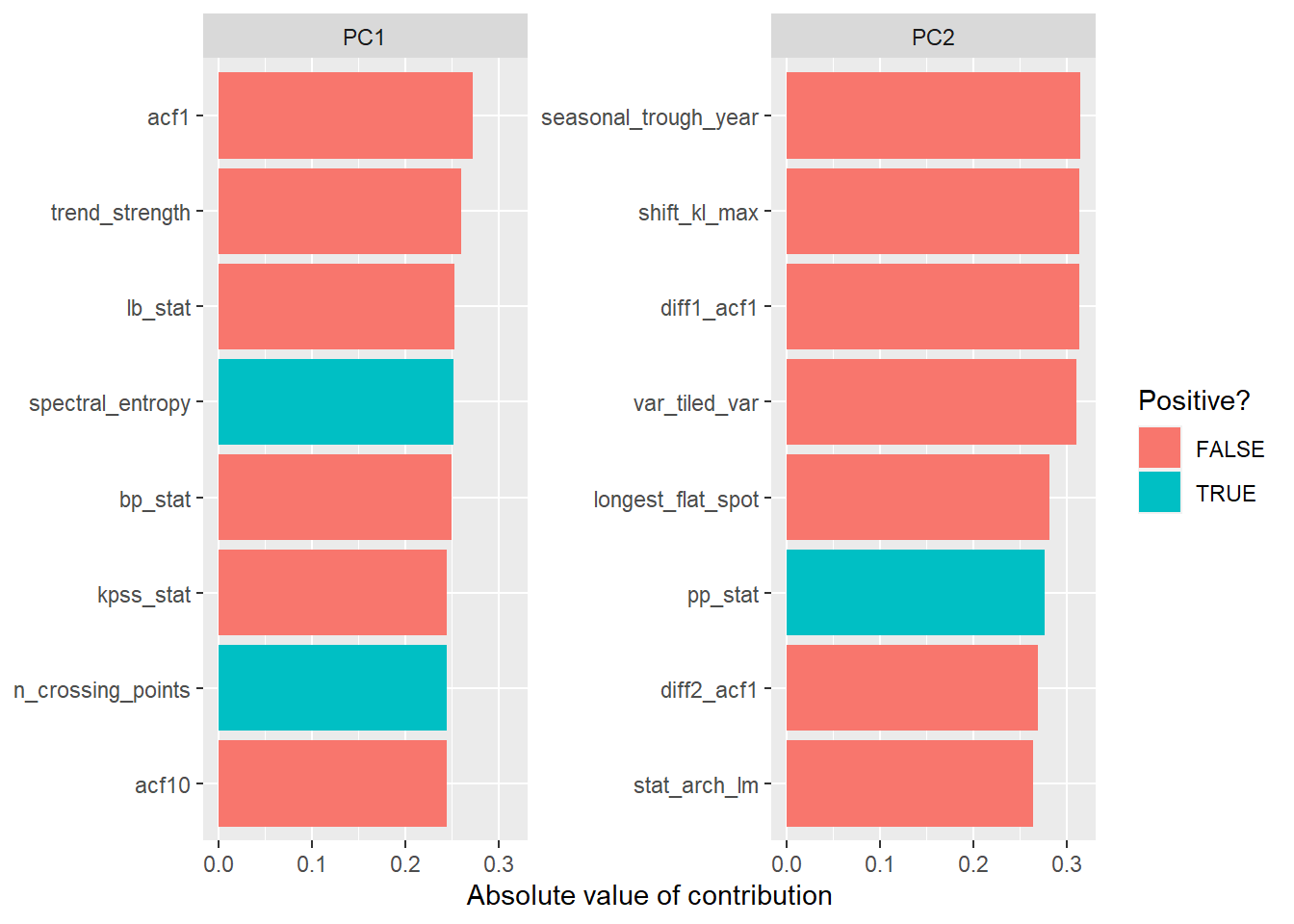
The first principal component captures 33% of the variance. PC1 is about
- trend & seasonality:
acf1(first ACF),acf10(sum of squared of first 10 ACF),trend_strength,spectral_entropy. - white noise:
lb_stat(Ljung-Box test),bp_stat(box_pierce),spectral_entropy
# https://juliasilge.com/blog/best-hip-hop/
library(tidytext)

feat_pca_PC %>%
  filter(component %in% paste0("PC", 1:2)) %>%
  group_by(component) %>%
  top_n(8, abs(value)) %>%
  ungroup() %>%
  mutate(terms = tidytext::reorder_within(terms, abs(value), component)) %>%
  ggplot(aes(abs(value), terms, fill = value > 0)) +
  geom_col() +
  facet_wrap(~component, scales = "free_y") +
  tidytext::scale_y_reordered() +
  labs(
    x = "Absolute value of contribution",
    y = NULL, fill = "Positive?"
  )
2.3 Distribution of hosptials in PC plane
feat_pca_df<-feat_pca_prep %>% bake(new_data=NULL)

feat_pca_df %>%
ggplot(aes(PC1, PC2, label = Name, colour=Name)) +
  geom_point() +
  ggrepel::geom_text_repel(force=.3)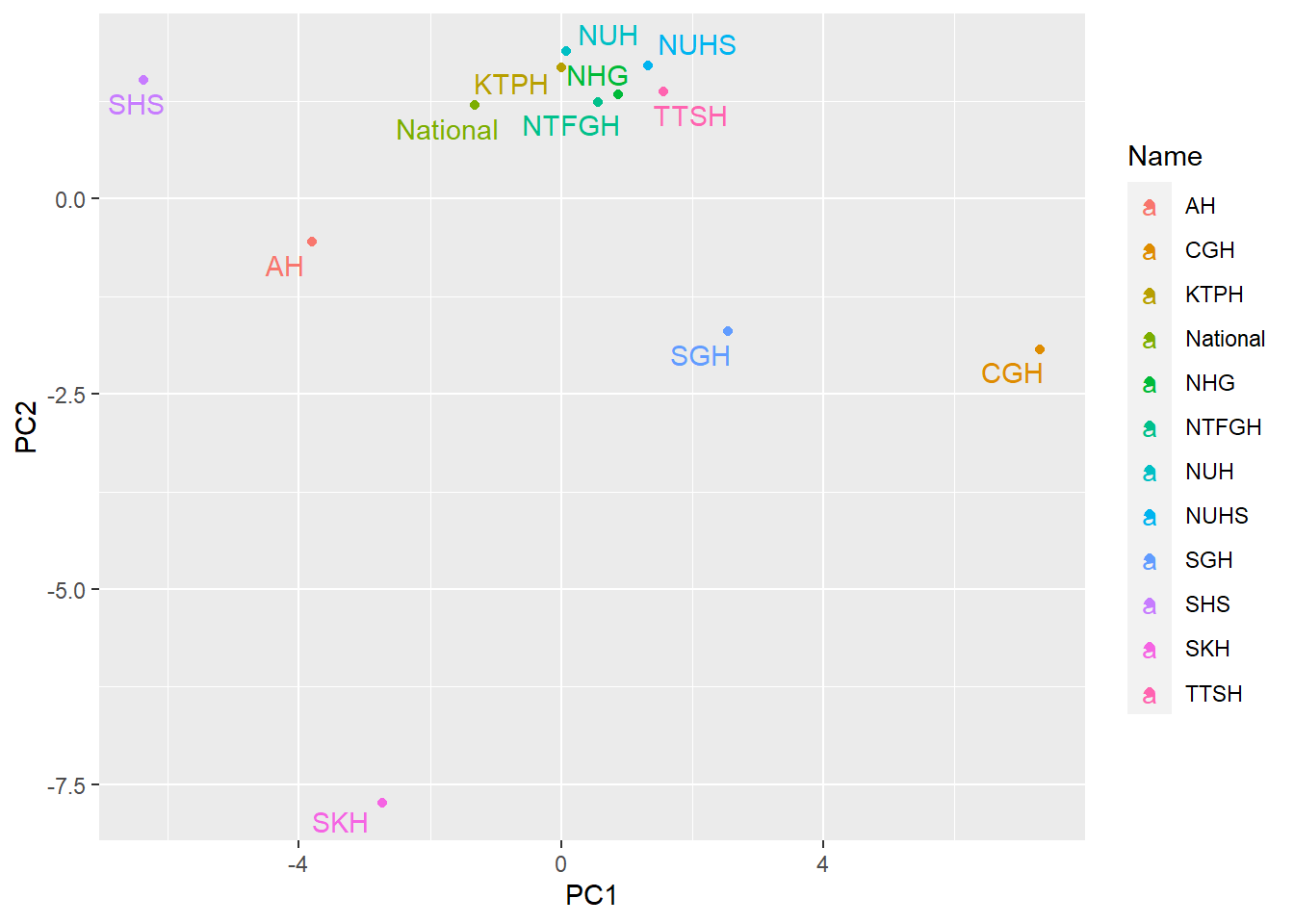
Conclusion
- There was an upward trend of admissions till the first half of 2020 which was flagged up as anomaly observations. => A dummy variable for this heightened COVID19 period would be considered when forecasting.
- Seasonality varied though a dipped in admissions during Feb was common => Seasonality should be included when forecasting.
- Lags varied (as sesaonlity varied too) => Lags should be considered when forecasting.
- Features of time series are heterogeneous and most of them moderately correlated => Include these features when forecasting especially with machine learning approach. Principal components of these features can also be used instead.
# add prefix for easier selection
feat_all<-feat_all %>% rename_with(~paste0("F_",.x), !c(Level, Name))

save(feat_all, file = "feat_all.RData")
Errors
Errors encountered during scripting.
1 Unable to use {{}} with as_tsibble
fun_ft<- function(k){
  mutate(Date= yearmonth(as.character(Date))) %>%
  as_tsibble(key= {{k}}, index= Date) %>%
  features(Admission, feature_set(pkgs="feasts"))
}

raw %>% fun_ft(Hospital)
## Error in fun_ft(., Hospital): unused argument (Hospital)