Explaining Predictions: Random Forest Post-hoc Analysis (randomForestExplainer package)
Recap
This is a continuation on the explanation of machine learning model predictions. Specifically, random forest models. We can depend on the random forest package itself to explain predictions based on impurity importance or permutation importance. Today, we will explore external packages which aid in explaining random forest predictions.
External packages
There are external a few packages which offer to calculate variable importance for random forest models apart from the conventional measurements found within the random forest package.
rfVarImpOOB
The first package is rfVarImpOOB which was recently released on CRAN. It “computes a novel variable importance for random forests”. Impurity reduction importance scores for out-of-bag data complements the existing in bag Gini importance. The vignette is unfortunately too brief in helping me understand the functions and the mechanism of this novel scoring of feature importance.
VSURF
The next package is VSURF which can handle high dimension datasets. It adopts a methodological three step approach to select important variables. Though there is no vignette, there is a BMC Medical Informatics and Decision Making research article using the VSURF package to look at features which are important to predict survival of individuals with breast cancer. The article explains the mechanism of how VSURF selects important features.
randomForestExplainer
The above journal article which used VSURF also used another package to select important features from a random forest. This other package is the randomForestExplainer. We will elaborate and demonstrate this package for the rest of the post. In the randomForestExplainer, the “various variable importance measures are calculated and visualized in different settings in order to get an idea on how their importance changes depending on our criteria”
Dataset
Similar to the previous posts, the Cleveland heart dataset will be used as well as principles of tidymodels.
#library
library(tidyverse)
library(tidymodels)
#import
heart<-read_csv("https://archive.ics.uci.edu/ml/machine-learning-databases/heart-disease/processed.cleveland.data", col_names = F)
# Renaming var
colnames(heart)<- c("age", "sex", "rest_cp", "rest_bp",
"chol", "fast_bloodsugar","rest_ecg","ex_maxHR","ex_cp",
"ex_STdepression_dur", "ex_STpeak","coloured_vessels", "thalassemia","heart_disease")
#elaborating cat var
##simple ifelse conversion
heart<-heart %>% mutate(sex= ifelse(sex=="1", "male", "female"),fast_bloodsugar= ifelse(fast_bloodsugar=="1", ">120", "<120"), ex_cp=ifelse(ex_cp=="1", "yes", "no"),
heart_disease=ifelse(heart_disease=="0", "no", "yes"))
## complex ifelse conversion using `case_when`
heart<-heart %>% mutate(
rest_cp=case_when(rest_cp== "1" ~ "typical",rest_cp=="2" ~ "atypical", rest_cp== "3" ~ "non-CP pain",rest_cp== "4" ~ "asymptomatic"), rest_ecg=case_when(rest_ecg=="0" ~ "normal",rest_ecg=="1" ~ "ST-T abnorm",rest_ecg=="2" ~ "LV hyperthrophy"), ex_STpeak=case_when(ex_STpeak=="1" ~ "up/norm", ex_STpeak== "2" ~ "flat",ex_STpeak== "3" ~ "down"), thalassemia=case_when(thalassemia=="3.0" ~ "norm",
  thalassemia== "6.0" ~ "fixed", thalassemia== "7.0" ~ "reversable"))
# convert missing value "?" into NA
heart<-heart%>% mutate_if(is.character, funs(replace(., .=="?", NA)))
# convert char into factors
heart<-heart %>% mutate_if(is.character, as.factor)
#train/test set
set.seed(4595)
data_split <- initial_split(heart, prop=0.75, strata = "heart_disease")
heart_train <- training(data_split)
heart_test <- testing(data_split)
Though random forest model itself doesn’t need explicit one hot encoding, some of randomForestExplainer functions need dummy variables. Thus we will create them in our recipe.
# create recipe object
heart_recipe<-recipe(heart_disease ~., data= heart_train) %>%
  step_knnimpute(all_predictors()) %>%
step_dummy(all_nominal(), -heart_disease)

# process the traing set/ prepare recipe(non-cv)
heart_prep <-heart_recipe %>% prep(training = heart_train, retain = TRUE)
In the randomForestExplainer vignette, computation of casewise importance measure was activiated (i.e. localImp=T). Likewise, we’ll do the same when we train our model.
set.seed(69)
rf_model<-rand_forest(trees = 2000, mtry = 4, mode = "classification") %>% set_engine("randomForest",
importance=T, localImp = T, ) %>% fit(heart_disease ~ ., data = juice(heart_prep))
randomForestExplainer (variable importance)
Measuring variable importance
The randomForestExplainer generates more feature importance score than the randomForest package. These scores generated by the randomForestExplainer::measure_importance function can be categorized into 3 types of feature importance score.
- Measures of importance based on the structure of the forest which is not examine in the
randomForestpackage.
1i) Mean_minimal_depth: Minimal depth for a variable in a tree equals to the depth of the node which splits on that variable and is the closest to the root of the tree. If it is low then a lot of observations are divided into groups on the basis of this variable.
1ii) no_of_nodes: Usually, number of trees and number of nodes are the same if trees are shallow. The number of nodes contain similar information as the number of trees and p-values. Thus, no_of_tress and p_value are omitted in plot_importance_ggpairs graph (which will be described later).
1iii) no_of_trees
1iv) p_value: Number of nodes in which predictor X was used for splitting exceeds the theoretical number of successes if they were random, following the binomial distribution given.
1v) times_a_root
- Measures of importance based on the decrease in predictive accuracy post variable perturbation
2i) accuracy_decrease: Use for classification problems. Same value as randomForest::importance(rf_model$fit, type=2)
2ii) mse_increase: Use for regression problems.
- Measure of importance based on loss function
3i) gini_decrease Use for classifcation cases. Same value as randomForest::importance(rf_model$fit, type=1).
3ii) node_purity_increase: Use for regression cases. Measured by the decrease in sum of squares
library(randomForestExplainer)
impt_frame<-measure_importance(rf_model$fit)

impt_frame %>% head()
## variable mean_min_depth no_of_nodes accuracy_decrease
## 1 age 3.076865 8635 0.004269917
## 2 chol 3.377786 8872 -0.003120879
## 3 coloured_vessels_X1.0 4.969157 3202 0.009133193
## 4 coloured_vessels_X2.0 4.155141 2600 0.010876652
## 5 coloured_vessels_X3.0 5.476794 1756 0.006136837
## 6 ex_cp_yes 3.791160 3033 0.009524295
## gini_decrease no_of_trees times_a_root p_value
## 1 8.686010 1979 54 0
## 2 7.997923 1983 3 0
## 3 2.814661 1749 13 1
## 4 3.769974 1675 82 1
## 5 2.044707 1280 20 1
## 6 5.557652 1766 187 1Ploting
plot_multi_way_importance plots variable importance scores from importance_frame. By default, the function plots scores measuring importance based on the structure of the forest, mean_min_depth against times_a_root.
plot_multi_way_importance(impt_frame, no_of_labels = 6)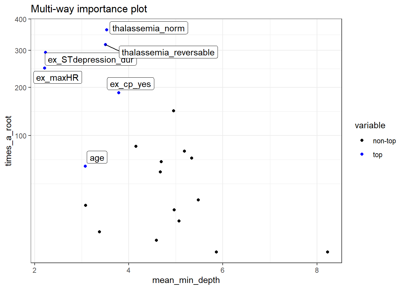
plot_multi_way_importance can plot up to 3 feature importance scores using any of the three kinds of importance measurements.
plot_multi_way_importance(impt_frame, x_measure = "accuracy_decrease", y_measure = "gini_decrease", size_measure = "p_value", no_of_labels = 6)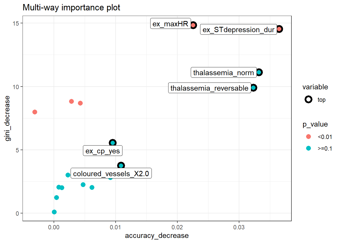
Selecting optimal importance scores to plot
There are many multi-way importance plots which one can create thus we need to identify which sub-set of importance scores will provide us with more helpful plots. Examining the relationship between the importance measurements with plot_importance_ggpairs can assist us in identifying a sub-set of scores to use. We can pick three scores that least agree with each other, points in plots which are most dispersed.
plot_importance_ggpairs(impt_frame)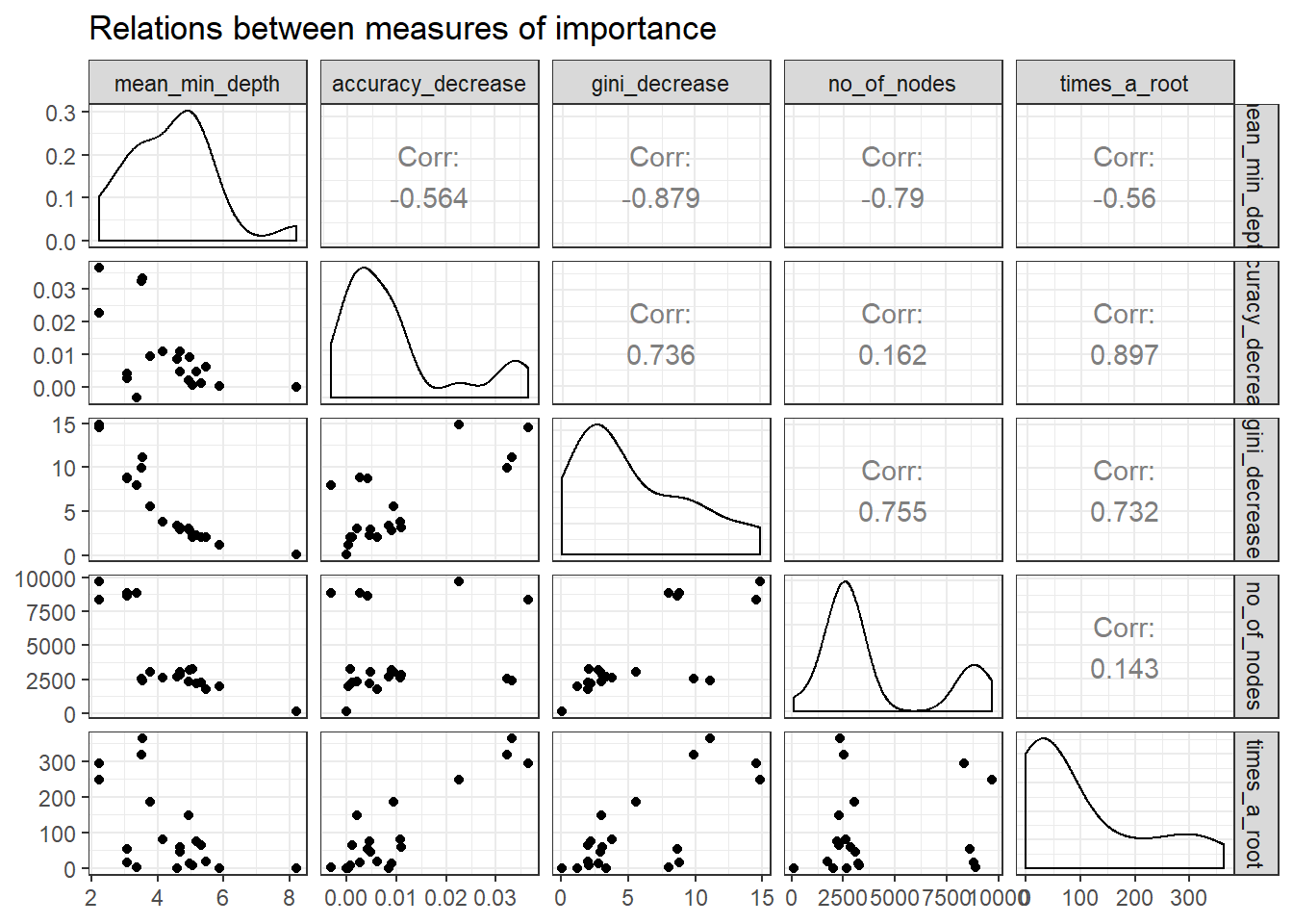 Plotting the rankings of importance measures with a LOESS curve using
 plot_importance_rankings informs us of pairs of measures almost exactly agreeing in their rankings of variables. This approach might be useful as rankings are more evenly spread than corresponding importance measures. This may also more clearly show where the different measures of importance disagree or agree.
plot_importance_rankings(impt_frame)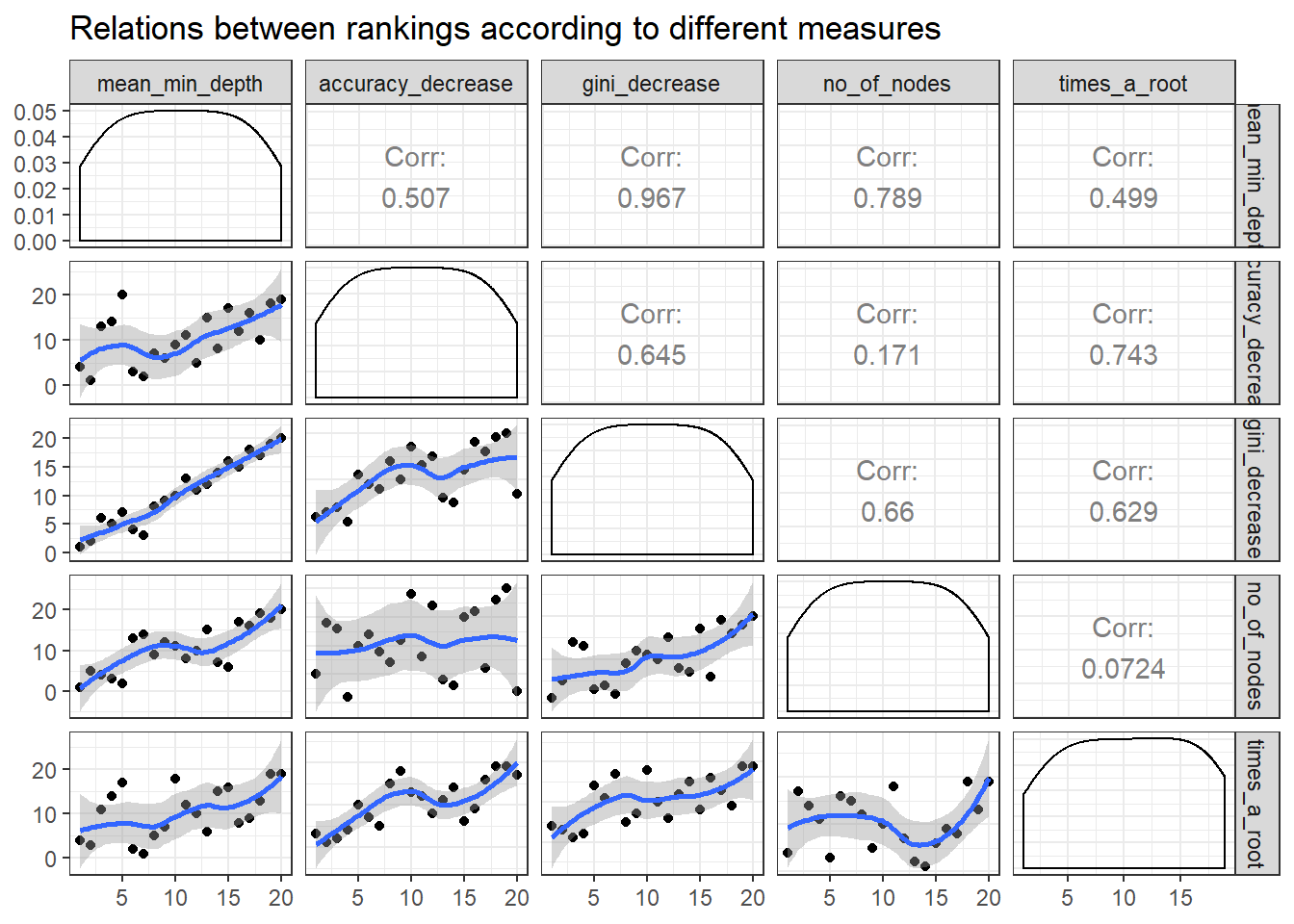
mean_min_depth and gini_decrease agree the most thus we should avoid this combination for plot_multi_way_importance.
randomForestExplainer: variable depth
Previously, we looked at various types of importance measures. Now we are specifically examining the mean minimal depth in detail. The distribution of the mean minimal depth allows us to appreciate the variable’s role in the random forest’s structure and prediction.
plot_min_depth_distribution plots the top ten variables according to mean minimal depth calculated using top trees.
The mean minimal depth can be calculated in 3 different ways in plot_min_depth_distribution using the mean_sample argument. The calculation differs in the way they treat missing values that appear when a feature is not used for tree splitting. As a result, the ranking of variables may change for each calculation.
md_frame <- min_depth_distribution(rf_model$fit)## Warning: Factor `split var` contains implicit NA, consider using
## `forcats::fct_explicit_na`plot_min_depth_distribution(md_frame, mean_sample = "top_trees") # default mean_sample arg 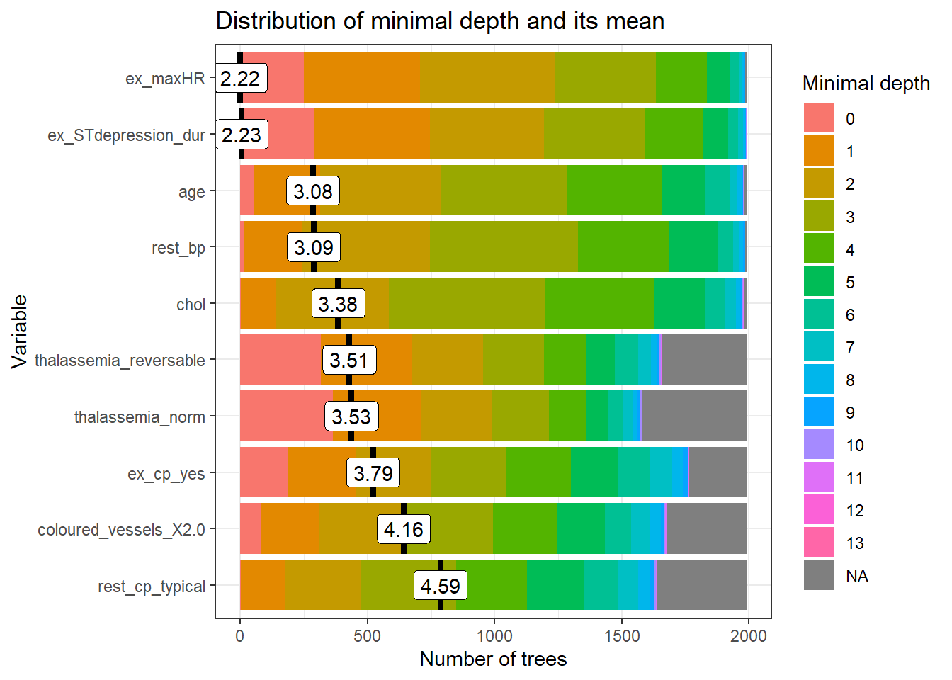 The mean minimal depth is indicated by a vertical bar with the mean value beside it. The smaller the mean minimal depth, the more important the variable is and the higher up the y-axis the variable will be.
The rainbow gradient reveals the min and max minimal depth for each variable. The bigger the proportion of minimal depth zero (red blocks), the more frequent the variable is the root of a tree. The smaller the proportion of NA minimal depth (gray blocks), the more frequent the variable is used for splitting trees.
The range of the x-axis is from zero to the maximum number of trees for the feature.
randomForestExplainer : variable interaction
We will use the important_variables function to select the top 6 variables based on the following variable importance measurements, times_a_root and no_of_nodes.
vars<- important_variables(impt_frame, k = 6, measures = c("times_a_root", "no_of_nodes"))After identifying the top 6 variables, we can examine the interactions between the variables with the min_depth_interactions function.
interactions_frame <- min_depth_interactions(rf_model$fit, vars)## Warning: Factor `split var` contains implicit NA, consider using
## `forcats::fct_explicit_na`
## Warning: Factor `split var` contains implicit NA, consider using
## `forcats::fct_explicit_na`The interaction is reflected as the mean_min_depth which is the mean conditional minimal depth, where a variable is taken as a root node/root_variable and the mean minimal depth is calculated for the other variable.
The uncond_mean_min_depth represents the unconditional mean minimal depth of the variable which is the mean minimal depth of the variable without having a stipulated root variable. This value is the same as the mean value seen on the vertical bar in plot_min_depth_distribution.
head(interactions_frame)## variable root_variable mean_min_depth occurrences
## 1 age age 2.766519 838
## 2 age ex_cp_yes 2.678235 940
## 3 age ex_maxHR 2.068416 1251
## 4 age ex_STdepression_dur 2.142738 1215
## 5 age thalassemia_norm 2.719905 1036
## 6 age thalassemia_reversable 2.539302 1064
## interaction uncond_mean_min_depth
## 1 age:age 3.076865
## 2 ex_cp_yes:age 3.076865
## 3 ex_maxHR:age 3.076865
## 4 ex_STdepression_dur:age 3.076865
## 5 thalassemia_norm:age 3.076865
## 6 thalassemia_reversable:age 3.076865We can plot the outputs from min_depth_interactions with plot_min_depth_interactions.
plot_min_depth_interactions(interactions_frame)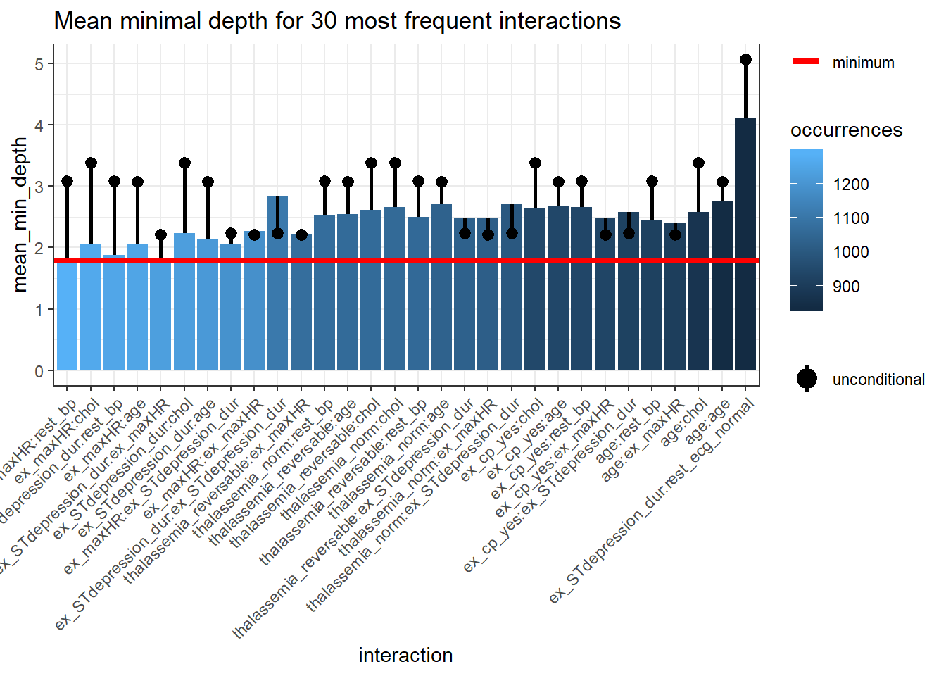 The interactions are arranged from the most frequent occurring on the left side of the plot and in lighter blue to the least frequent occurring interaction on the right side of the plot and in darker blue.
The horizontal red line represents the minimum
 mean_min_depth.
The black lollipop represents the uncond_mean_min_depth.
Similar to plot_min_depth_distribution, the ranking of interactions in plot_min_depth_interactions may change depending on the arguments for mean_sample and uncond_mean_sample.
Interactive variables and forest prediction
We can further evaluate the variable interactions by plotting the probability of a prediction against the variables making up the interaction. For instance we plot the probability of having heart disease against resting blood pressure rest_bp and ST depression duration during exercise test ex_STdepression_dur. The interaction of these two variables are the most frequent interaction as seen in plot_min_depth_interactions. We plot the forest prediction against interactive variables with plot_predict_interaction.
#plot_predict_interaction(rf_model$fit, bake(heart_prep, new_data = heart_train), "rest_bp", "ex_STdepression_dur")However, there is an error when the input supplied is a model created with parsnip. There is no error when the model is created directly from the randomForest package.
set.seed(69)
forest <- randomForest::randomForest(heart_disease ~ ., data = bake(heart_prep, new_data = heart_train), localImp = TRUE, importance=T, ntree = 2000, mtry = 4, type= "classification")
plot_predict_interaction(forest, bake(heart_prep, new_data = heart_train), "rest_bp", "ex_STdepression_dur", main = "Distribution of Predicted Probability of Having Heart Disease") + theme(legend.position="bottom") + geom_hline(yintercept = 2, linetype="longdash") + geom_vline(xintercept = 140, linetype="longdash")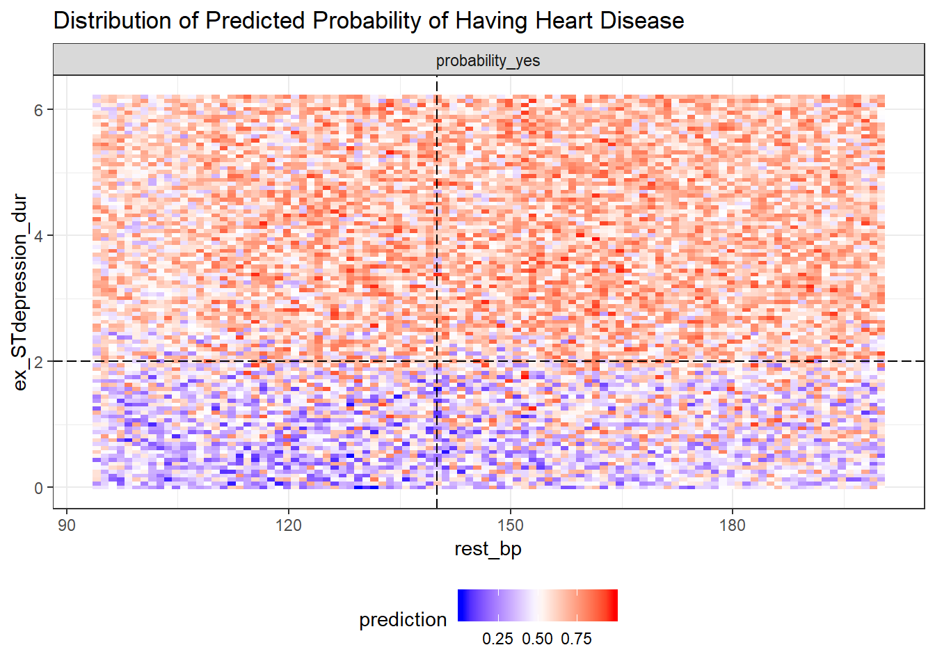 ST depression duration during exercise test
 ex_STdepression_dur longer than 2s results in higher predicted probability of having a heart disease. The predicted probability of having heart disease for individuals with shorter ST depression duration (<2s) increases if they have high resting blood pressure rest_bp above 140.
As plot_predict_interaction is a ggplot object which you can treat it like any other ggplot. In this case, we can place it side by side with the ggplot of the distribution of heart disease in the test set.
predict_plot<-plot_predict_interaction(forest, bake(heart_prep, new_data = heart_train), "rest_bp", "ex_STdepression_dur", main = "Distribution of Predicted\n Probability of Having Heart\n Disease") + theme(legend.position="bottom") + geom_hline(yintercept = 2, linetype="dotted")

test_plot<-ggplot(heart_test, aes(rest_bp, ex_STdepression_dur, colour=heart_disease)) +geom_jitter(size=1.8) + labs(title="Distribution of Heart Disease\n in Test Set", y="") + theme_minimal() +  scale_color_manual(values=c("blue", "red")) +  theme(legend.position="bottom") + geom_hline(yintercept = 2, linetype="dotted")

gridExtra::grid.arrange(predict_plot, test_plot, ncol=2)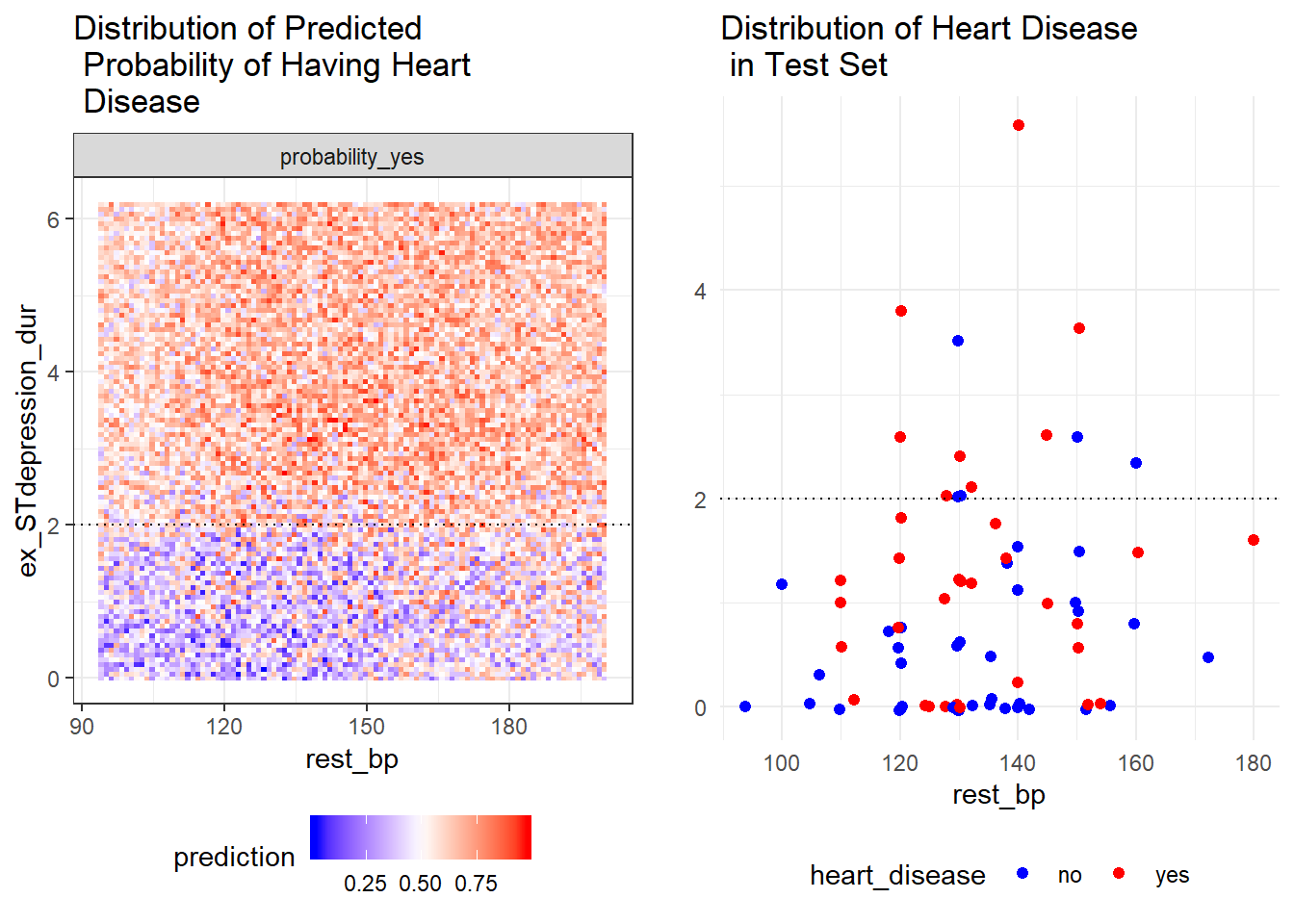
Conclusion
In this post, we learned how random forest predictions can be explained based on various variable importance measures, variable interactions and variable depth. The post-hoc analysis was aided with the randomForestExplainer package.
Comments
thalaseemia_norm,thalassemia_reversable,ex_maxHRandex_STdepression_durappear in both plots. These variables are more likely to be essential in the random forest’s prediction.thalaseemia_normandthalassemia_reversableare identified as one of the six variables with goodgini_decreaseandaccuracy_decreasebut they are insignificant asp_value>=.1.