Predicting pneumonia outcomes: EDA part 1
- Intro
- 1
Other_related category - 2
Pt_Patient related category - 3
R_Radiology related category - 4
SS_Category related to signs and symptoms of CAP - 5
Hx_medical history category - 6
Social_social history category - 7
HCAP_healthcare associated pneumonia category - 8
PE_observations during physical examination category - To be continued….
This post is a supplementary material for an assignment. The assignment is part of the Augmented Machine Learning unit for a Specialised Diploma in Data Science for Business. The aim of the assignment is to use DataRobot for predictive modelling. Exploratory data analysis and feature engineering will be done here in R before the data is imported into DataRobot.
Intro
The dataset is from a prospective population-based surveillance study. For reproducibility, use this spreadsheet as I have appended
extra sheets to the orginal spreadsheet used by the researchers. Metadata to sheet 2 (metadata) and a description of each category to sheet 3 (Category). The observational study was conducted over 3 different South America cities across 3 different countries over a 3-year period to investigate the incidence rate of Community Acquired Pneumonia (CAP). The dataset has a wealth of variables which can be used for predictive modelling, there is no known predictive analysis published using this dataset. The aim of this project is to classify if patients with CAP became better after seeing a doctor or became worse despite seeing a doctor.
library(tidyverse)
theme_set(theme_light())

raw<- readxl::read_excel("Incidence rate of community-acquired pneumonia in adults a population-based prospective active surveillance study in three cities in South America.xls")
## Warning in read_fun(path = enc2native(normalizePath(path)), sheet_i = sheet, :
## Expecting logical in EL1372 / R1372C142: got '2014-09-02'## Warning in read_fun(path = enc2native(normalizePath(path)), sheet_i = sheet, :
## Expecting logical in EM1372 / R1372C143: got '2014-09-08'The dataset consists of 2302 rows and 176 columns.
dim(raw)## [1] 2302 176The original column names were the description of the variables (e.g. Received flu shot in the last 12 months). Based on these descriptions/column names, the columns can be classified into 13 categories (see table below). Most of the categories ae clinically related variables.
categories13<- readxl::read_excel("Incidence rate of community-acquired pneumonia in adults a population-based prospective active surveillance study in three cities in South America.xls", sheet=3)

categories13 %>%  DT::datatable(rownames = F, options = list(searchHighlight = TRUE, paging= T))
Data dictionary
The column names are renamed to shorter column names (e.g. Received flu shot in the last 12 months-> flu) with prefixes to identify which of the above 13 categories they belong to (e.g. flu-> V_flu. Prefix V_ stands for vaccine against the flu.).
metadata<- readxl::read_excel("Incidence rate of community-acquired pneumonia in adults a population-based prospective active surveillance study in three cities in South America.xls", sheet=2)

# metadata
metadata %>%  DT::datatable(rownames = F, options = list(searchHighlight = TRUE, paging= T))
# rename col names
colnames(raw)<- metadata$`New column name` %>% t()EDA blueprint
EDA will be iterated for each of the 13 categories as there are too many columns to do the EDA at once. Also, there may be some association among the variables for each category. EDA includes exploring (i) the types of variables for each category (ii) the number of missing values (iii) the number of outliers (iv) and data cleaning if needed. Customized functions were created to facilitate EDA:
dtypeprovides the number of columns beginning with the prefix (e.g.dtype(dataframe, “Pt”)will list all the columns related to patient (pt). The types of variables are also provided.eda_cbreaks down the labels for columns beginning with the prefix. Used mostly for categorical variables.eda_n_NApltplots the percentage ofNA/missing values for each column beginning with the prefix. Used mostly for numeric variables.eda_n_NAcutoffprovides a vector of variable names with acceptableNAvalues. Used mostly for numeric variables. The ball park maximum amount of missing values is 20% though higher proportion of missing values may be included after inspecting the plot generated byeda_n_NAplteda_n_outlierplots boxplots for numeric variables beginning with the prefix. Variables with large number of outliers can be isolated for further investigation.
dtype<- function(datafr, x){
datafr %>% select(starts_with(x, ignore.case = F)) %>% str()
}

eda_c<- function(datafr,x){
  datafr %>% select(starts_with(x, ignore.case = F)) %>%  map(~ table(.x, useNA = "always"))
}

eda_n_NAplt<- function (datafr, x){
  datafr %>% select(starts_with(x, ignore.case = F)) %>% summarise(across(starts_with(x), ~mean(is.na(.)))) %>% pivot_longer(cols = everything(), names_to= "Variables" , values_to="pct_na") %>% mutate(Variables= fct_reorder(Variables, pct_na)) %>% ggplot(aes(x=Variables, y=pct_na, fill= pct_na))+ geom_col() + coord_flip() + scale_y_continuous(labels=scales::percent_format()) + scale_fill_viridis_c(option = "plasma")}

eda_n_NAcutoff<- function(datafr, x, low, high){
  datafr%>% select(starts_with(x, ignore.case = F)) %>% summarise(across(starts_with(x), ~mean(is.na(.)))) %>% pivot_longer(cols = everything(), names_to="Variables", values_to="pct_na") %>% filter((pct_na>low & pct_na<high)) %>% pull(Variables)}

eda_n_outlier<-function(datafr, x_selected){
# nested df with plots
  plt<-datafr %>% select(all_of(x_selected)) %>% pivot_longer(cols=everything(),names_to="Variables", values_to="values") %>% nest(-Variables) %>% mutate(plot= map2(.x= data, .y= Variables,
~ggplot(data=.x, aes(x= values)) + geom_boxplot() + labs(title = .y)
))
# print the plots
  for (i in 1:length(x_selected)){
    p<-plt[[3]][[i]]
    print(p)}
  }
Outcome
The outcome will be Other_Outcome. As the prediction is whether the patient was better or worse after seeking medical treatment, a binary classification is warranted here. However the Other_Outcome has 4 values, namely cure, improvement, unfavourable and death.
eda_c(raw, "Other_Outcome")## $Other_Outcome
## .x
## Cure death Improvement unfavorable <NA>
## 799 277 1179 26 21cure and improvement will be collapsed as better and unfavourable and death will be collapsed as worse. 6 times as many patients became better after seeking medical help. While encouraging from the doctor’s and patient’s perspective, it results in an imbalanced dataset for prediction. The imbalanced dataset will be addressed much later.
After removing 21 NA outcomes, there are 2281 observations remaining.
# collapse 4 categories into 2
raw$Other_Outcome<-fct_collapse(raw$Other_Outcome, better=c("Cure", "Improvement"))
raw$Other_Outcome<-fct_collapse(raw$Other_Outcome, worse=c("unfavorable", "death"))

# remove na
df<-raw %>%  filter(!is.na(Other_Outcome))
eda_c(df, "Other_Outcome")
## $Other_Outcome
## .x
## better worse <NA>
## 1978 303 0Discard the noise
There are column names with the prefix rm_ in front of the category prefix (e.g. rm_Other_). These columns are removed for numerous reasons.
dtype(df,"rm")## tibble [2,281 x 36] (S3: tbl_df/tbl/data.frame)
## $ rm_R_CXR : chr [1:2281] "Yes" "Yes" "Yes" "Yes" ...
## $ rm_R_CT : chr [1:2281] "No" "No" "No" "No" ...
## $ rm_R_CT_date : chr [1:2281] NA NA NA NA ...
## $ rm_SS : logi [1:2281] NA NA NA NA NA NA ...
## $ rm_SS_infilterate : chr [1:2281] "Yes" "Yes" "Yes" "Yes" ...
## $ rm_SS_WBC : chr [1:2281] "Yes" "Yes" "No" "No" ...
## $ rm_HCAP : chr [1:2281] "No" "No" "No" "No" ...
## $ rm_PE : logi [1:2281] NA NA NA NA NA NA ...
## $ rm_PE_O2 : chr [1:2281] "Yes" "Yes" "Yes" "Yes" ...
## $ rm_Lab : logi [1:2281] NA NA NA NA NA NA ...
## $ rm_Lab_RBC : chr [1:2281] "Yes" "Yes" "Yes" "Yes" ...
## $ rm_Lab_Hb : chr [1:2281] "Yes" "Yes" "Yes" "Yes" ...
## $ rm_Lab_WBC : chr [1:2281] "Yes" "Yes" "Yes" "Yes" ...
## $ rm_Lab_NeuImu : chr [1:2281] "No" "No" "No" "No" ...
## $ rm_Lab_NeuImuDate : chr [1:2281] NA NA NA NA ...
## $ rm_Lab_Neu : chr [1:2281] "Yes" "Yes" "Yes" "Yes" ...
## $ rm_Lab_plt : chr [1:2281] "Yes" "Yes" "Yes" "Yes" ...
## $ rm_Lab_Na : chr [1:2281] "No" "No" "No" "No" ...
## $ rm_Lab_NaDate : chr [1:2281] NA NA NA NA ...
## $ rm_Lab_urea : chr [1:2281] "Yes" "No" "Yes" "Yes" ...
## $ rm_Lab_Cr : chr [1:2281] "Yes" "No" "Yes" "Yes" ...
## $ rm_Lab_Bicarb : chr [1:2281] "No" "No" "No" "No" ...
## $ rm_Lab_BicarbDate : chr [1:2281] NA NA NA NA ...
## $ rm_Lab_Sugar : chr [1:2281] "Yes" "No" "Yes" "Yes" ...
## $ rm_Lab_Alb : chr [1:2281] "No" "No" "No" "No" ...
## $ rm_Lab_AlbDate : chr [1:2281] NA NA NA NA ...
## $ rm_Lab_lactate : chr [1:2281] "No" "No" "No" "No" ...
## $ rm_Lab_lactateDate : chr [1:2281] NA NA NA NA ...
## $ rm_Lab_CRP : chr [1:2281] "Yes" "Yes" "No" "Yes" ...
## $ rm_Lab_ABG : chr [1:2281] "No" "No" "No" "No" ...
## $ rm_Lab_ABGDate : chr [1:2281] NA NA NA NA ...
## $ rm_Abx : logi [1:2281] NA NA NA NA NA NA ...
## $ rm_Care_ICUdate : chr [1:2281] NA NA NA NA ...
## $ rm_Other_phone : chr [1:2281] "Yes" "Yes" "Yes" "Yes" ...
## $ rm_Other_1yearstatus: chr [1:2281] "dead after 1 year" NA "dead after 1 year" "dead after 1 year" ...
## $ rm_Abx_AbxDuration : chr [1:2281] "Yes" "Yes" "Yes" "Yes" ...For instance, 1 year status contains information about the patient’s status one year post CAP which is a data leakage as it reveals the patient’s outcome from the CAP.
df %>% select(rm_Other_1yearstatus) %>% tail()## # A tibble: 6 x 1
## rm_Other_1yearstatus
## <chr>
## 1 alive
## 2 dead after 1 year
## 3 alive
## 4 alive
## 5 alive
## 6 aliveOther columns contained duplicated information. For lab results, there is a column, which indicates if the specific biochemical was tested (eg rm_Lab_urea), and another column of the result (eg Lab_urea). If the biochemical was not tested, the column will indicate No test being done and the result column will be blank. Keeping only the results column will suffice. The reasons for removing specific rm_ columns is described in the above data dictionary.
df %>% select(rm_Lab_urea, Lab_urea) %>% head()## # A tibble: 6 x 2
## rm_Lab_urea Lab_urea
## <chr> <dbl>
## 1 Yes 60
## 2 No NA
## 3 Yes 99
## 4 Yes 56
## 5 Yes 143
## 6 Yes 56.3The dataframe of 176 columns ends up with 140 columns after discarding rm_ columns.
df<-df %>% select(-starts_with("rm"))

ncol(df)
## [1] 1405 Hx_ medical history category
(dtype(df, "Hx"))## tibble [2,281 x 17] (S3: tbl_df/tbl/data.frame)
## $ Hx_mass : chr [1:2281] "No" "No" "No" "No" ...
## $ Hx_heart : chr [1:2281] "No" "No" "Yes" "Yes" ...
## $ Hx_stroke : chr [1:2281] "No" "No" "No" "No" ...
## $ Hx_kidney : chr [1:2281] "No" "No" "No" "No" ...
## $ Hx_liver : chr [1:2281] "No" "No" "No" "No" ...
## $ Hx_brainMental : chr [1:2281] "No" "No" "No" "No" ...
## $ Hx_diabetes : chr [1:2281] "No" "No" "No" "No" ...
## $ Hx_pastCAP : chr [1:2281] "No" "No" "No" "No" ...
## $ Hx_asp : chr [1:2281] "Yes" "No" "No" "No" ...
## $ Hx_alcohol : chr [1:2281] "No" "No" "No" "No" ...
## $ Hx_immune : chr [1:2281] "No" "No" "No" "No" ...
## $ Hx_COPD : chr [1:2281] "No" "Yes" "No" "No" ...
## $ Hx_heart_type : chr [1:2281] NA NA NA NA ...
## $ Hx_HIV : chr [1:2281] "No" "No" "No" "No" ...
## $ Hx_HIV_CD4 : num [1:2281] NA NA NA NA NA NA NA NA NA NA ...
## $ Hx_HIV_viralLoad: chr [1:2281] NA NA NA NA ...
## $ Hx_HIV_Medicine : chr [1:2281] "Unavailable" "Unavailable" "Unavailable" "Unavailable" ...## NULL(eda_c(df,"Hx"))## $Hx_mass
## .x
## No Uncertain Yes <NA>
## 2152 9 117 3
##
## $Hx_heart
## .x
## No Uncertain Yes <NA>
## 1273 19 983 6
##
## $Hx_stroke
## .x
## No Uncertain Yes <NA>
## 2105 11 161 4
##
## $Hx_kidney
## .x
## No Uncertain Yes <NA>
## 2110 7 156 8
##
## $Hx_liver
## .x
## No Uncertain Yes <NA>
## 2214 4 58 5
##
## $Hx_brainMental
## .x
## No Uncertain Yes <NA>
## 1907 28 341 5
##
## $Hx_diabetes
## .x
## No Uncertain Yes <NA>
## 1907 13 358 3
##
## $Hx_pastCAP
## .x
## No Uncertain Yes <NA>
## 1985 5 287 4
##
## $Hx_asp
## .x
## No Uncertain Yes <NA>
## 2202 15 59 5
##
## $Hx_alcohol
## .x
## No Uncertain Yes <NA>
## 2117 18 135 11
##
## $Hx_immune
## .x
## No Uncertain Yes <NA>
## 2130 4 139 8
##
## $Hx_COPD
## .x
## No Uncertain Yes <NA>
## 1879 50 343 9
##
## $Hx_heart_type
## .x
## Arrhythmia CHF Hypertension
## 23 43 220
## Isquemic cardiomyopathy Other <NA>
## 20 1 1974
##
## $Hx_HIV
## .x
## No Unavailable Yes <NA>
## 2134 105 42 0
##
## $Hx_HIV_CD4
## .x
## 14 41 74 99 127 175 245 291 324 349 485 493 844 1104 <NA>
## 1 1 1 3 1 1 1 1 1 1 1 1 1 1 2265
##
## $Hx_HIV_viralLoad
## .x
## < Detection limit > Detection limit Value <NA>
## 5 3 4 2269
##
## $Hx_HIV_Medicine
## .x
## No Unavailable Yes <NA>
## 596 1671 14 0HIV details
Remove Hx_HIV_CD4 & Hx_HIV_viralLoad as there are too many NA. Remove Hx_HIV_Medicine as there are too many Unavailable.
df<-df %>% select(-contains("Hx_HIV_"))Heart disease
Hx_heart indicates whether the patient has heart disease or not. Hx_heart_type provides details on the type of heart disease. Both the variables can be integrated into a variable.
1273 observations for heart disease details, Hx_heart_type were labelled as NA not because they are truly missing but because these patients have No heart disease. These values will be labelled as None. 19 observations for heart disease details were labelled as NA when the heart disease status is Uncertain. These values will be labelled as Query heart disease. 676 observations for heart disease details were labelled as NA but were classified to have a heart disease. As these patients have heart diseases but no details can be obtained, the NA values will be treated as Other types of heart disease.
After using Hx_heart to expand Hx_heart_type, Hx_heart will be dropped.
(table(df$Hx_heart, df$Hx_heart_type, useNA="always"))##
## Arrhythmia CHF Hypertension Isquemic cardiomyopathy Other <NA>
## No 0 0 0 0 0 1273
## Uncertain 0 0 0 0 0 19
## Yes 23 43 220 20 1 676
## <NA> 0 0 0 0 0 6# relabel
df<- df %>% mutate(Hx_heart_type=case_when(
Hx_heart== "No" & is.na(Hx_heart_type) ~ "None",
Hx_heart=="Uncertain" & is.na(Hx_heart_type) ~ "Query heart disease",
Hx_heart=="Yes" & is.na(Hx_heart_type) ~ "Other",
T~ Hx_heart_type))
(table(df$Hx_heart, df$Hx_heart_type, useNA="always"))##
## Arrhythmia CHF Hypertension Isquemic cardiomyopathy None Other
## No 0 0 0 0 1273 0
## Uncertain 0 0 0 0 0 0
## Yes 23 43 220 20 0 677
## <NA> 0 0 0 0 0 0
##
## Query heart disease <NA>
## No 0 0
## Uncertain 19 0
## Yes 0 0
## <NA> 0 6# remove `hx_heart`
df <- df %>% select (-Hx_heart)7 HCAP_ healthcare associated pneumonia category
No data cleaning is needed for this category.
(dtype(df,"HCAP"))## tibble [2,281 x 5] (S3: tbl_df/tbl/data.frame)
## $ HCAP_hospStay: chr [1:2281] "Yes" "No" "No" "No" ...
## $ HCAP_IVAbx : chr [1:2281] "No" "No" "No" "No" ...
## $ HCAP_Chemo : chr [1:2281] "No" "No" "No" "No" ...
## $ HCAP_diaylsis: chr [1:2281] "No" "No" "No" "No" ...
## $ HCAP_injury : chr [1:2281] "No" "No" "No" "No" ...## NULL(eda_c(df, "HCAP"))## $HCAP_hospStay
## .x
## No Uncertain Yes <NA>
## 2039 3 236 3
##
## $HCAP_IVAbx
## .x
## No Uncertain Yes <NA>
## 2074 1 203 3
##
## $HCAP_Chemo
## .x
## No Uncertain Yes <NA>
## 2240 3 33 5
##
## $HCAP_diaylsis
## .x
## No Uncertain Yes <NA>
## 2234 1 41 5
##
## $HCAP_injury
## .x
## No Uncertain Yes <NA>
## 2206 3 63 98 PE_ observations during physical examination category
(dtype(df, "PE"))## tibble [2,281 x 7] (S3: tbl_df/tbl/data.frame)
## $ PE_AMS : chr [1:2281] "No" "No" "No" "Unavailable" ...
## $ PE_HR : num [1:2281] 88 92 100 95 95 110 85 85 110 85 ...
## $ PE_RR : num [1:2281] 26 24 48 30 30 28 26 25 26 28 ...
## $ PE_BP_S: num [1:2281] 100 110 140 140 120 140 100 120 120 100 ...
## $ PE_BP_D: num [1:2281] 50 60 80 80 60 90 60 60 80 60 ...
## $ PE_temp: num [1:2281] 38 38 36 37 36 39 37 37 40 37 ...
## $ PE_O2 : chr [1:2281] NA NA NA NA ...## NULL# explore categorical
(eda_c(df, "PE_AMS"))## $PE_AMS
## .x
## No Unavailable Yes <NA>
## 1832 29 420 0Oxygen levels, PE_O2 are calculated in the form of percentage. In this case, there is a mixture of pure numbers and numbers ending with % resulting in the variable to be treated as a character variable. % will be omitted and the variable will be converted to a numeric variable.
(eda_c(df, "PE_O2"))## $PE_O2
## .x
## 100 37 55 58
## 3 1 1 1
## 60 63 65 67
## 3 1 3 1
## 7 70 73 74
## 1 9 3 6
## 75 76 77 78
## 3 2 3 10
## 79 80 80.099999999999994 82
## 4 23 1 18
## 83 84 85 85 %
## 12 17 23 2
## 86 86,7 86.599999999999994 87
## 21 1 1 19
## 88 88% 88,9 88.900000000000006
## 55 1 1 1
## 89 90 91 91.299999999999997
## 50 116 62 1
## 92 92% 92.400000000000006 93
## 124 1 1 107
## 93 % 93.400000000000006 93.599999999999994 94
## 1 1 1 153
## 94 % 94.299999999999997 94.5 95
## 1 1 1 153
## 95.5 95.609999999999999 95.900000000000006 96
## 1 1 1 191
## 96 % 96.5 96.700000000000003 97
## 1 1 1 142
## 97.5 98 99 <NA>
## 1 97 35 784# clean up `PE_O2`
df<-df %>% mutate(PE_O2= as.numeric(str_replace_all(PE_O2,pattern="%", replacement = "")))## Warning in mask$eval_all_mutate(dots[[i]]): NAs introduced by coercionMissing PE_ values
Now, all the PE_ variables are in numeric form and the proportion of NA can be appropriately calculated. Oxygen levels PE_O2 has the highest proportion of missing values, >30% values are missing. PE_O2 will be dropped.
(eda_n_NAplt(df,"PE"))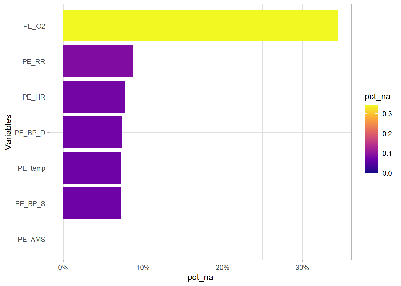
df<-df %>% select(-PE_O2)Outlier PE_ values
The following variables have unrealistic outliers:
- Temperature,
PE_temp. Outliers >50’C will be explored - Breathing rate,
PE_RR. Outliers of >50 breaths per minute will be explored - Diastolic blood pressure,
PE_BP_D. There is only one observation with a diastolic blood pressure >300, this observation will be removed.
pe_selected<-eda_n_NAcutoff(df, "PE", 0, 0.3)

(eda_n_outlier(df,pe_selected))
## Warning: All elements of `...` must be named.
## Did you want `data = c(values)`?## Warning: Removed 176 rows containing non-finite values (stat_boxplot).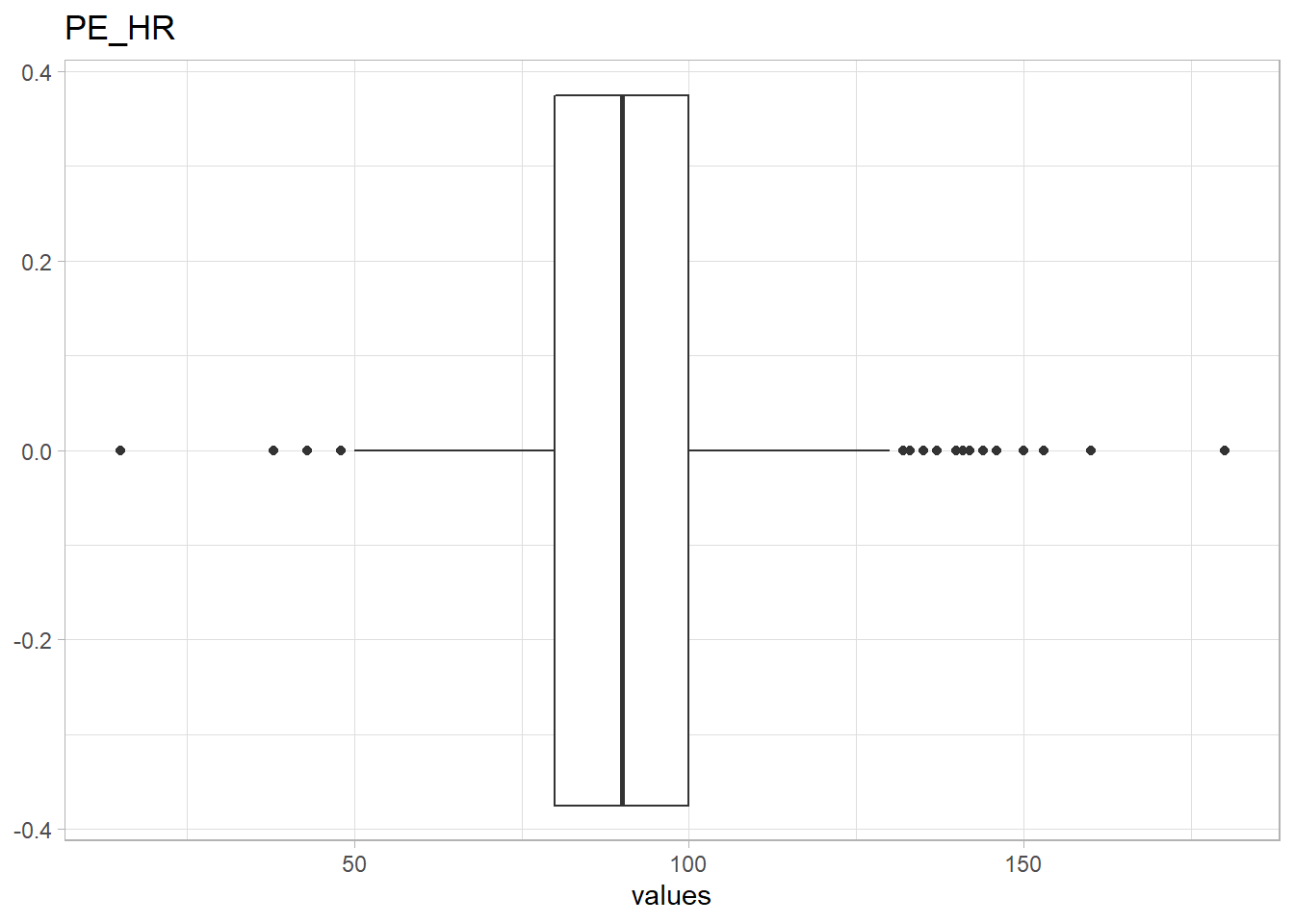
## Warning: Removed 201 rows containing non-finite values (stat_boxplot).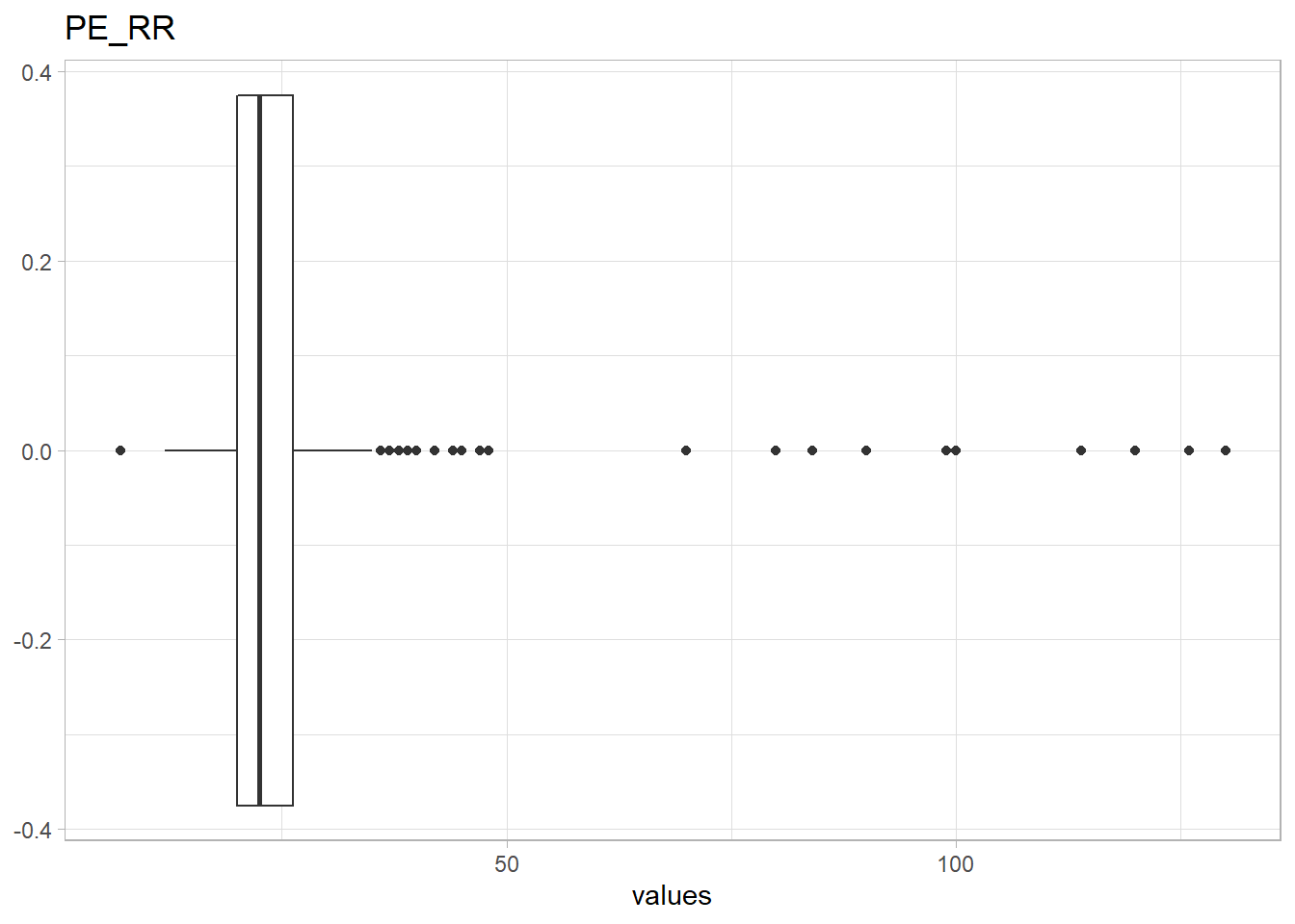
## Warning: Removed 167 rows containing non-finite values (stat_boxplot).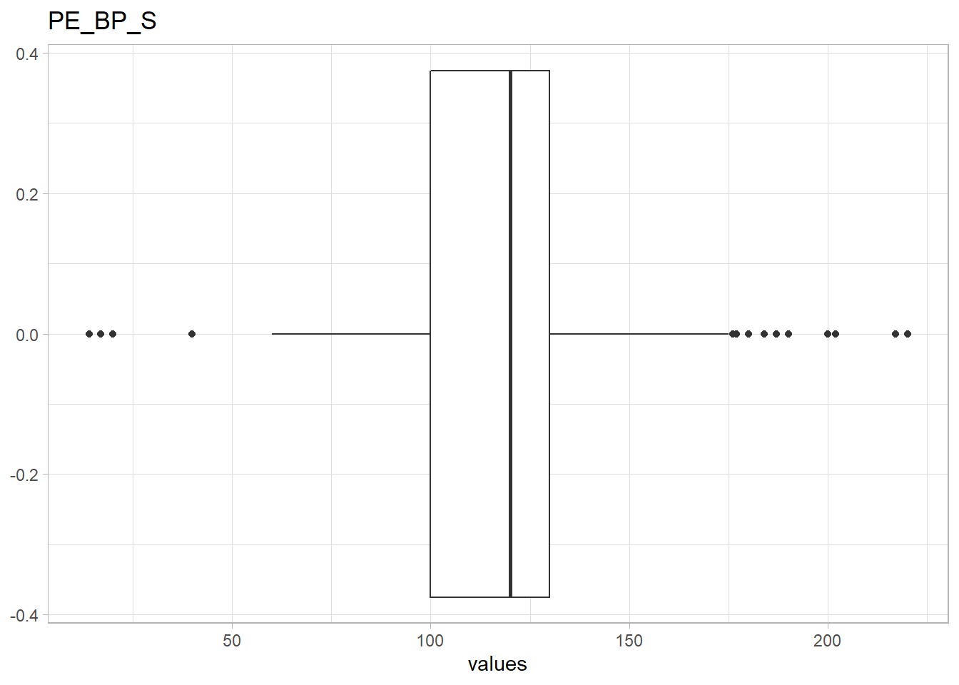
## Warning: Removed 168 rows containing non-finite values (stat_boxplot).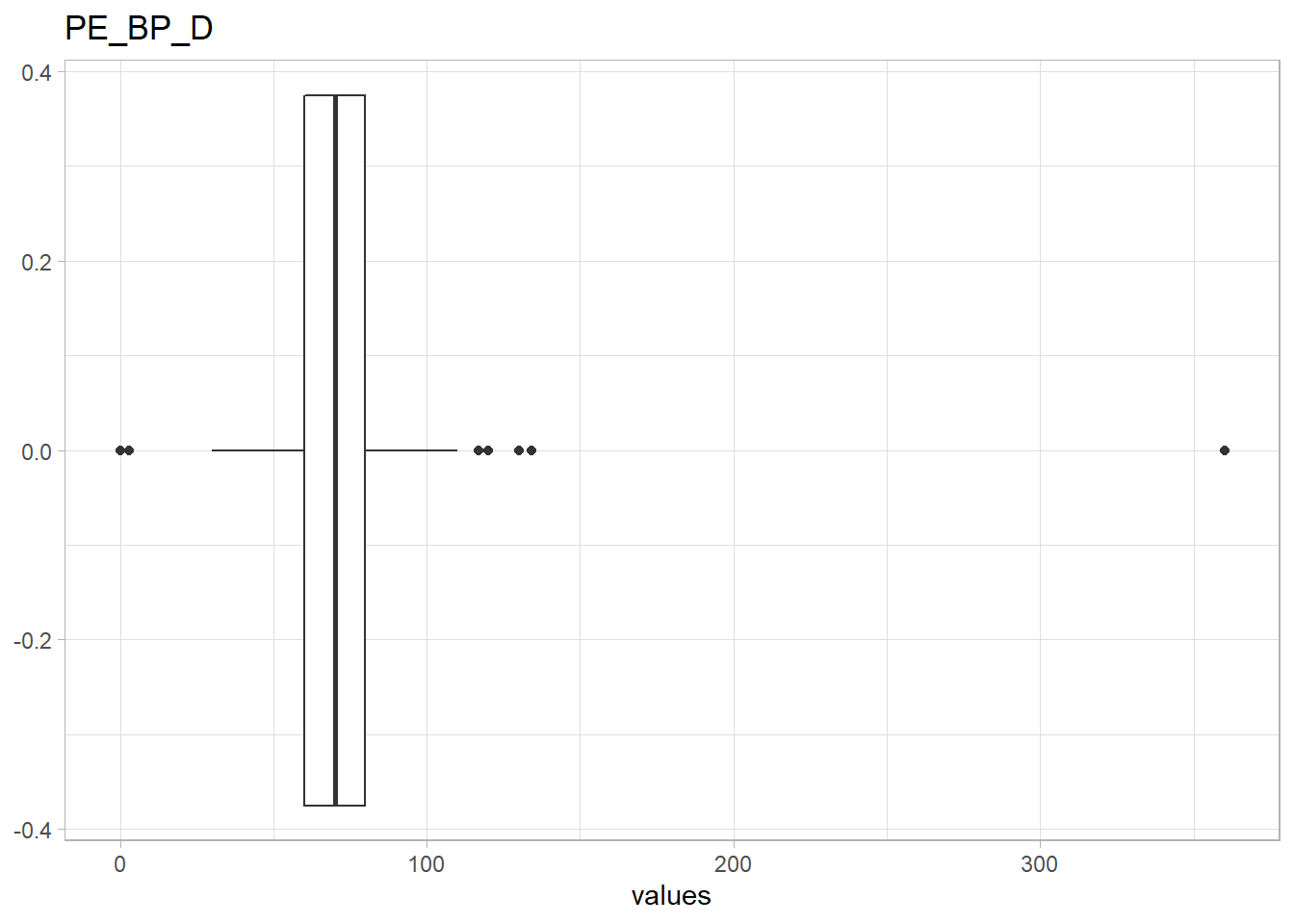
## Warning: Removed 167 rows containing non-finite values (stat_boxplot).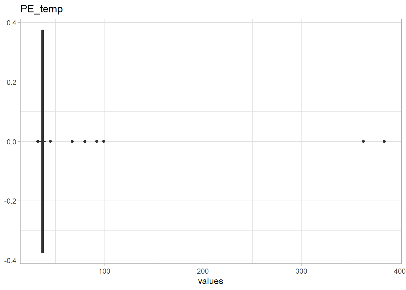
## NULLdf<-df %>% filter(PE_BP_D<300)Further investigation of outliers
The 90-ish values stand out for both PE_temp and PE_RR. A frequency count will be done.
(df %>% filter(PE_temp>50) %>% ggplot(aes(PE_temp)) + geom_histogram(bins=round(sqrt(nrow(df)))))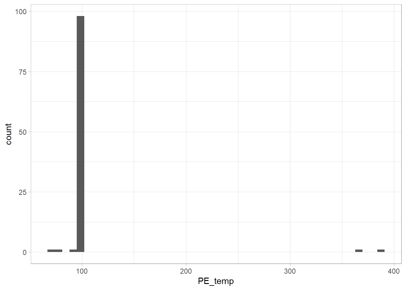
(df %>% filter(PE_RR>50) %>% ggplot(aes(PE_RR)) + geom_histogram(bins=round(sqrt(nrow(df)))))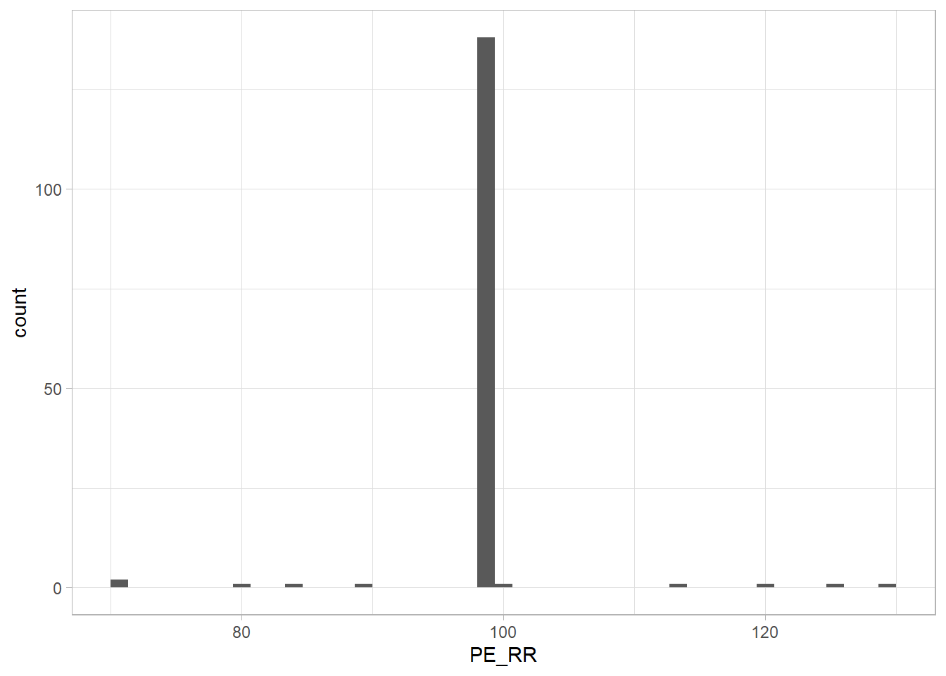
99 is the most common value. Similar to previous numeric variables where 99 is an outlier, it will be converted to NA. For PE_temp, the values 363 and 384, are likely missing a decimal point (It is more likely your body’s temperature is 36.3’C instead of 363’C) .
# PE_temp
(df %>% filter(PE_temp>50) %>% group_by(PE_temp) %>% summarise(n(), .groups="drop"))
## # A tibble: 6 x 2
## PE_temp `n()`
## <dbl> <int>
## 1 67 1
## 2 80 1
## 3 92 1
## 4 99 98
## 5 363 1
## 6 384 1# PE_RR
(df %>% filter(PE_RR>50) %>% group_by(PE_RR) %>% summarise(n(), .groups="drop"))## # A tibble: 10 x 2
## PE_RR `n()`
## <dbl> <int>
## 1 70 2
## 2 80 1
## 3 84 1
## 4 90 1
## 5 99 138
## 6 100 1
## 7 114 1
## 8 120 1
## 9 126 1
## 10 130 1The rest of the outliers will take a plausible maximum value based on the 90th-95th percentile.
# 90-ish percentile
(quantile(df$PE_temp, probs = seq(0,1,.05), na.rm = T))
## 0% 5% 10% 15% 20% 25% 30% 35% 40% 45% 50% 55% 60% 65% 70% 75%
## 32 36 36 36 36 36 36 37 37 37 37 37 37 38 38 38
## 80% 85% 90% 95% 100%
## 38 38 39 40 384(quantile(df$PE_RR, probs = seq(0,1,.05), na.rm = T))## 0% 5% 10% 15% 20% 25% 30% 35% 40% 45% 50% 55% 60% 65% 70% 75%
## 7 16 16 18 18 20 20 20 21 22 23 24 24 24 26 27
## 80% 85% 90% 95% 100%
## 28 30 35 99 130# clean up PE_temp and PE_RR
df<-df %>% mutate(PE_temp=na_if(PE_temp, 99), PE_RR=na_if(PE_RR, 99),
PE_temp=if_else(PE_temp==363, 36.3, PE_temp), PE_temp=if_else(PE_temp==384, 38.4, PE_temp),
PE_temp=if_else(PE_temp>50, 40, PE_temp), PE_RR=if_else(PE_RR>50, 35, PE_RR)) To be continued….
Before this post becomes too long, EDA for the remaining categories
- lab findings
Lab_ - cultures
CS_ - antibiotics
Abx_ - continiuum of care state
Care_ - vaccine
V_
will be done in the next post.
save(df, file = "CAP_EDA1.RData")
6
Social_social history categorysmoking
Social_smokeindicates if the patient smokes or not.Social_smoke_durationrecords how long the patients was smoking. These variables contain different facets of the same information; the values can be integrated into a single column.1276 observations for smoking duration,
Social_smoke_durationwere labelled asNAbut these values were not truly missing. These patients did not smoke. The values will be relabelled asnon-smoker. 175 observations for smoking duration were labelled asNAbut the information if they smoked wasUnavailable. These values will be relabelled asUnavailable. All the patients who smoked had the duration of their smoking habit recorded. The bins of smoking duration were relabelled to terms that are more intuitive.currentwas relabelled asstill smokes,In the last 5 yearswas relabelled assmoked in the last 5y,Previous to the last 5 yearswas relabelled assmoked >5y ago.After using
Social_smoketo expandSocial_smoke_duration,Social_smokeis dropped.