Intro

This post is a supplementary material for an assignment. The assignment is part of the Augmented Machine Learning unit for a Specialised Diploma in Data Science for Business. The aim of the assignment is to use DataRobot for predictive modelling. Exploratory data analysis and feature engineering will be done here in R before the data is imported into DataRobot. The aim of this project is to classify if patients with Community Acquired Pneumonia (CAP) became better after seeing a doctor or became worse despite seeing a doctor.
In the 2 previous posts (part1, part2), a dataset on Community Acquired Pneumonia was explored and cleaned up. In this post, some feature engineering will be done.

library(tidyverse)
#https://github.com/notast/pneumonia-outcomes/blob/master/pneumonia_EDA2.Rmd
load("CAP_EDA2.RData")
theme_set(theme_light())

plt_common<- function(datafr, var, glued_title, s_title){
  datafr %>% mutate(var_reordered =fct_reorder({{var}}, rel))%>%
    ggplot(aes(var_reordered, rel, fill=rel)) + geom_col() + coord_flip() +  scale_fill_viridis_c(option = "cividis", alpha = .5) +
scale_y_continuous(labels=scales::percent_format()) + labs(title= glue::glue(glued_title), subtitle = s_title, x="")}

Antibiotics used

The goal is to have a frequency breakdown on the types of antibiotics used and lump the infrequent types of antibiotics used.

Patients who were not prescribed antibiotics will be separated for this analysis

df_abx<-df %>% filter(Abx_no!=0)
df_abxNo<-df %>% filter(Abx_no==0)

Currently, the type of antibiotics used is displayed as binary variables in a wide format.

df %>% select(Abx_AmoxicillinSulbactam:Abx_OtherYN) %>% head()

## # A tibble: 6 x 17
##   Abx_Amoxicillin~ Abx_Amoxicillin~ Abx_Amoxicillin~ Abx_Ampicillin
##   <chr>            <chr>            <chr>            <chr>         
## 1 No               No               No               No            
## 2 Yes              No               No               No            
## 3 Unavailable      Unavailable      Unavailable      Unavailable   
## 4 No               No               No               No            
## 5 No               No               No               No            
## 6 No               No               No               No            
## # ... with 13 more variables: Abx_AmpicillinSulbactam <chr>,
## #   Abx_Azithromycin <chr>, Abx_Ceftriaxone <chr>, Abx_Cefotaxime <chr>,
## #   Abx_ClarithromycinOral <chr>, Abx_Cefepime <chr>,
## #   Abx_ClarithromycinIV <chr>, Abx_Doxycycline <chr>, Abx_Levofloxacin <chr>,
## #   Abx_Moxifloxacin <chr>, Abx_Piperacillin <chr>, Abx_Trimethoprim <chr>,
## #   Abx_OtherYN <chr>

Additionally, the details of other types of antibiotics used is stored in a different column, Abx_OtherDetail.

df %>% select(Abx_OtherYN, Abx_OtherDetail) %>% tail(10)

## # A tibble: 10 x 2
##    Abx_OtherYN Abx_OtherDetail
##    <chr>       <chr>          
##  1 No          <NA>           
##  2 Yes         Cefuroxime     
##  3 Yes         Clindamycin    
##  4 No          <NA>           
##  5 No          <NA>           
##  6 No          <NA>           
##  7 No          <NA>           
##  8 No          <NA>           
##  9 No          <NA>           
## 10 No          <NA>

The dataframe will need to be pivoted to a long dataframe. The values of Abx_OtherDeail will be used during wrangling to have a complete set on types of antibiotics used in the study.

long_df<-df %>% pivot_longer(cols = Abx_AmoxicillinSulbactam:Abx_OtherYN, "Abx_type", values_to= "Used") %>% 
  #abx prescribed
  filter(Used=="Yes") %>% 
  # integrate details from Abx_OtherDetail to expand type of abx used for "Abx_OtherYN"
mutate(Abx_type=case_when(
    Abx_type=="Abx_OtherYN" & !is.na(Abx_OtherDetail) ~ Abx_OtherDetail, 
    Abx_type=="Abx_OtherYN" & is.na(Abx_OtherDetail) ~ "Abx_unknown",
    T~Abx_type
  ),
  Abx_type= str_remove(Abx_type, "Abx_"),
  Abx_type= str_glue("Abx_{Abx_type}")) %>% 
  # `Abx_OtherDetail` is now redundant 
  select(-Abx_OtherDetail)

50 antibiotics were used in the study and most of them were rarely used.

# plot 
(long_df %>% 
   # rel frequ
  count(Abx_type) %>% mutate(rel=prop.table(n)) %>% 
  plt_common(Abx_type, "{n_distinct(long_df %>% pull(Abx_type))} antibiotics were prescribed", ""))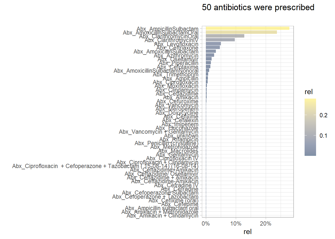

# tabuluar
(long_df %>% filter(Used=="Yes") %>% count(Abx_type) %>% mutate(rel=prop.table(n)) %>% 
arrange(-rel) %>% select(Abx_type, rel))

## # A tibble: 50 x 2
##    Abx_type                        rel
##    <glue>                        <dbl>
##  1 Abx_AmpicillinSulbactam      0.279 
##  2 Abx_AmoxicillinSulbactamOral 0.237 
##  3 Abx_ClarithromycinOral       0.128 
##  4 Abx_ClarithromycinIV         0.0962
##  5 Abx_Levofloxacin             0.0501
##  6 Abx_Ceftriaxone              0.0466
##  7 Abx_AmoxicillinSulbactam     0.0330
##  8 Abx_Azithromycin             0.0276
##  9 Abx_Oseltamivir              0.0187
## 10 Abx_Piperacillin             0.0165
## # ... with 40 more rows

Only the top 9 antibiotics will be kept and the less frequent antibiotics will be lumped together.

long_df<- long_df %>%  mutate(Abx_type= fct_lump_n(Abx_type, n=9, other_level = "Abx_LowFreq"))

long_df%>% filter(Used=="Yes") %>%  count(Abx_type) %>% mutate(rel=prop.table(n)) %>% 
  plt_common(Abx_type, "Top 9 antibiotics", "Low frequency antibiotics were outside the top 9 and were lumped together")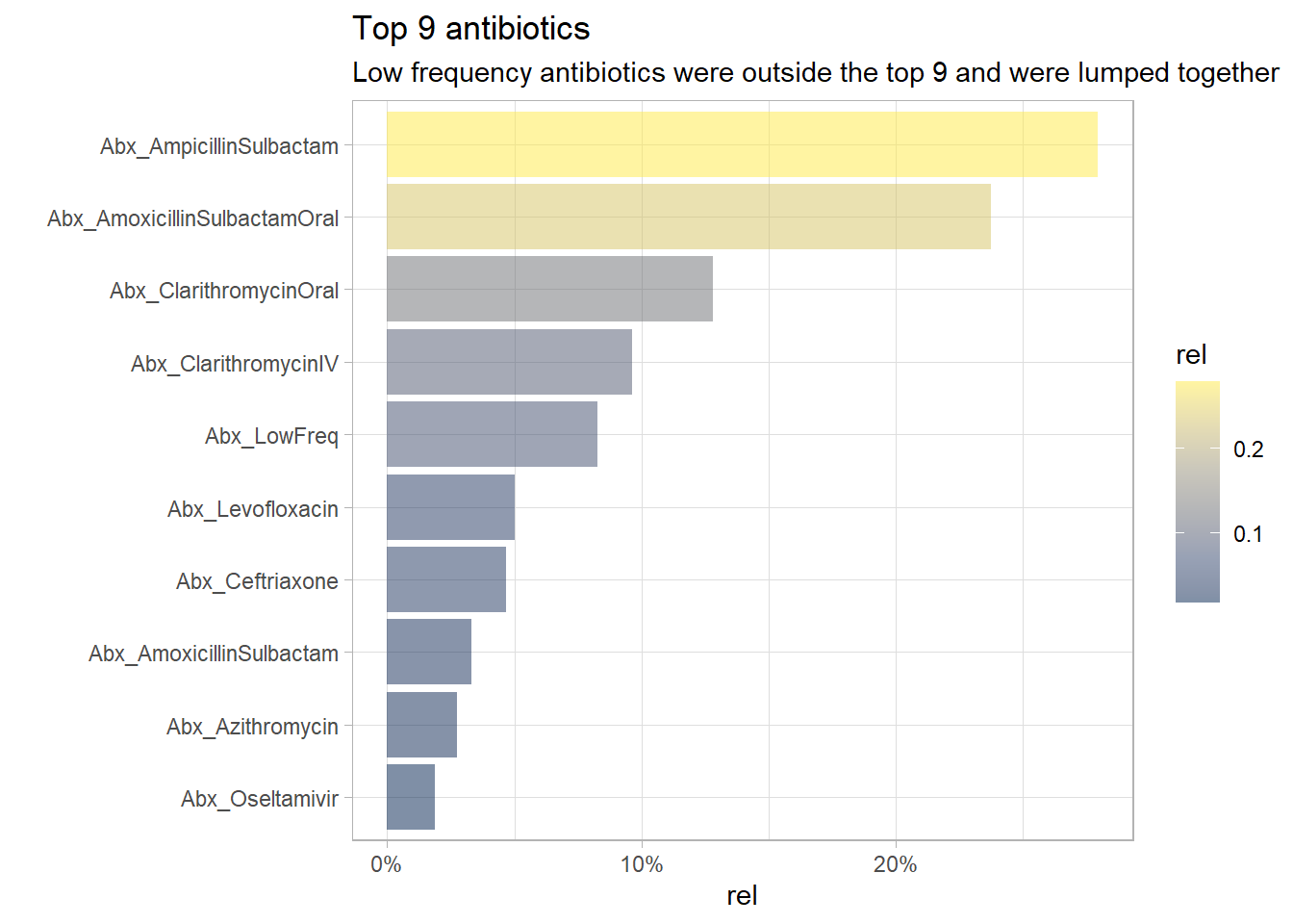 

Class of empirical antibiotics used

Similarly, the goal is to lump the infrequent empirical antibiotics class. 30 empirical antibiotics class were used in the study, most of them were rarely used.

(long_df %>% count(Abx_ClassUpdated) %>% mutate(rel=prop.table(n)) %>% 
  plt_common(Abx_ClassUpdated, "{n_distinct(long_df %>% pull(Abx_ClassUpdated))} empirical antibiotics class used", ""))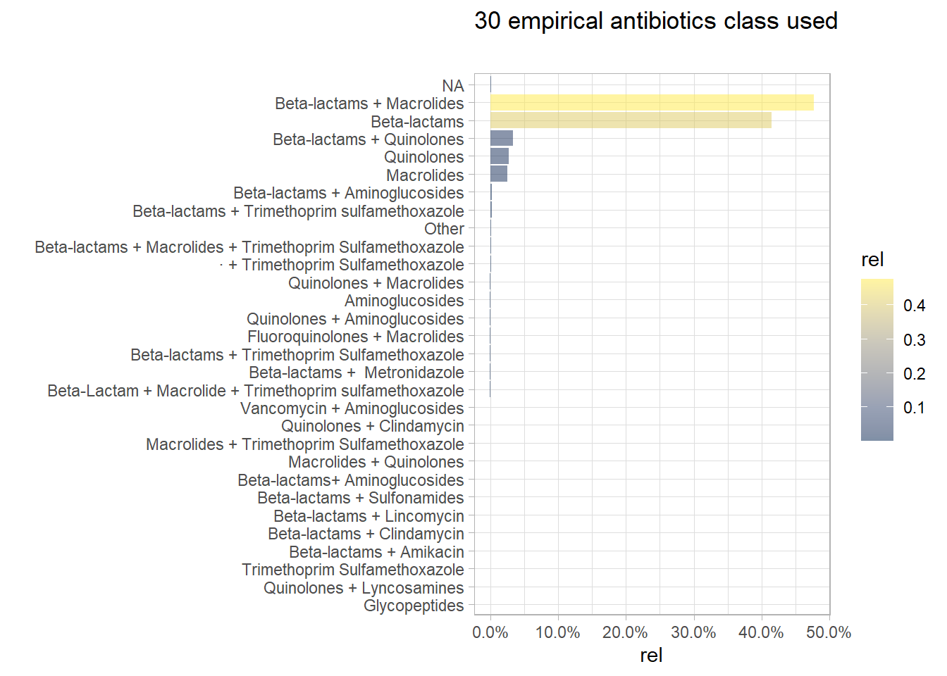

Only the top 4 classes will be kept and the less frequent classes will be lumped together. There is a small proportion of NA antibiotics class which will be imputed. An alternative was to review the antibiotics prescribed and use clinical knowledge to deduce the empirical antibiotic prescribed and therefore providing information of the class of empirical antibiotics used.

# lump abx_class 
long_df<- long_df %>% mutate(Abx_ClassUpdated= fct_lump_n(Abx_ClassUpdated , n= 4, other_level = "Low freq"))

# re-plot 
long_df %>% count(Abx_ClassUpdated) %>% mutate(rel=prop.table(n)) %>% 
  plt_common(Abx_ClassUpdated, "Top 4 empirical antibiotic class", "Low frequency class were outside the top 4 and were lumped together")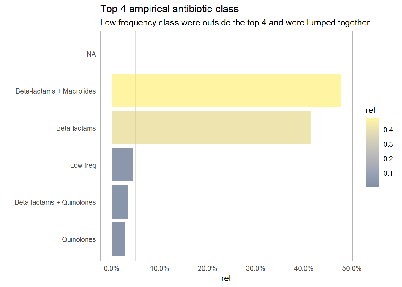

Lastly, the long dataframe will be spread into the original wide format and the patients who were not prescribed antibiotics are added back into the dataframe

df2<-long_df %>% pivot_wider(names_from = Abx_type, values_from=Used,
# may have multiple `yes` for Abx_LowFreq due to lumping. need to summarise with `unique` to remove duplicate `yes` OR use `length` to to count the number of low freq abx used
                        values_fn={Abx_LowFreq= length},
                        values_fill=0) 

# add pt w/o abx
df2<-bind_rows(df_abxNo %>% select(-starts_with("Abx")), 
         df2) %>% 
  mutate(Abx_ClassUpdated=replace_na(as.character(Abx_ClassUpdated), "No Abx"),
         across(.cols= (Abx_Duration:Abx_ClarithromycinIV), .fns = ~replace_na(.x, 0)),
         # num binary -> y/n binary for abx 
         across(.cols=(c(Abx_Ceftriaxone, Abx_AmoxicillinSulbactam:Abx_ClarithromycinIV)), .fns=~if_else(.x==1, "Yes", "No")))

Feature Enginnering

Additional features will be created based on the available variables and clinical knowledge.

# Get the breakdown of Pt_site
eda_c<- function(datafr,x){
  datafr %>% select(starts_with(x, ignore.case = F)) %>%  map(~ table(.x, useNA = "always"))
}

(eda_c(df2, "Pt_Site"))

## $Pt_Site
## .x
## Location A Location B Location C       <NA> 
##        241       1042        829          0

# map the site 
df2<-  df2 %>% mutate(Pt_Site= case_when(
    Pt_Site=="Location A"~ "Concepción_PY", 
  Pt_Site=="Location B"~"GeneralRoca_AR",
  Pt_Site=="Location C"~ "Rivera_UY"
  ))  %>% # include weather 
mutate(Pt_climate=case_when(
  Pt_Site == "Concepción_PY" | Pt_Site=="Rivera_UY" ~"subtropical",
  Pt_Site== "GeneralRoca_AR"~"cold windy"
  )) %>% relocate(Pt_climate, .after=Pt_Site)

(df2 %>% select(Pt_Site, Pt_climate) %>% sample_n(10))

## # A tibble: 10 x 2
##    Pt_Site        Pt_climate 
##    <chr>          <chr>      
##  1 Concepción_PY  subtropical
##  2 Rivera_UY      subtropical
##  3 Rivera_UY      subtropical
##  4 GeneralRoca_AR cold windy 
##  5 GeneralRoca_AR cold windy 
##  6 Rivera_UY      subtropical
##  7 Rivera_UY      subtropical
##  8 GeneralRoca_AR cold windy 
##  9 GeneralRoca_AR cold windy 
## 10 GeneralRoca_AR cold windy

Comorbidities

Based on the patient’s past medical history Hx_, the number of comorbidities can be calculated. calculated. Patients with CAP and comorbidities have been shown to have poorer outcomes. However, there are missing values in Hx which need to be imputed first.

plt_na<-function(dfr, X, t, st){
  dfr  %>% summarise(across(starts_with(X), ~mean(is.na(.)))) %>% pivot_longer(cols = everything(), names_to= "Variables" , values_to="pct_na") %>% mutate(Variables= fct_reorder(Variables, pct_na)) %>% ggplot(aes(x=Variables, y=pct_na, fill= pct_na))+ geom_col() + coord_flip() + scale_y_continuous(labels=scales::percent_format()) + scale_fill_viridis_c(option = "plasma") + labs(title = t, subtitle = st)}

plt_na(df2, "Hx", "before imputation", NULL)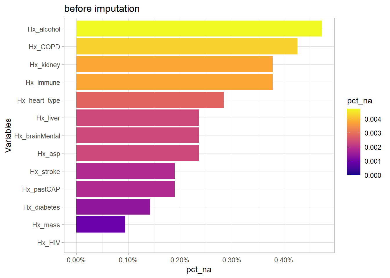

library(recipes)
set.seed(69)
df3<-recipe(Outcome ~., data= df2) %>%  update_role(Pt_CaseNumber, new_role = "id variable") %>%  step_bagimpute(starts_with("Hx")) %>% prep() %>% juice()

plt_na(df3,"Hx","post imputation", "imputed with decision trees")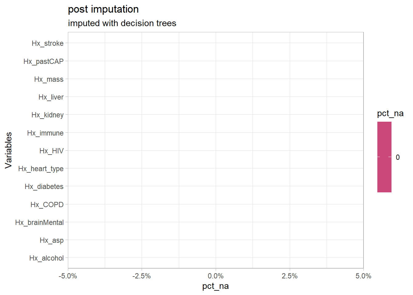

The comorbidities can now be calculated

df3<-df3 %>% mutate(
  # collapse various heart disease to `yes`
  Hx_heart_type= if_else(Hx_heart_type =="None", "None", "Yes"),
  # convert y/n to binary numbers. need numeric for calculation
  across(.cols=starts_with("Hx"), .fns = ~if_else(.x=="Yes", 1,0))) %>% 
  # calculate comorbidities
  rowwise() %>% 
  mutate(Hx_comorbidities= sum(c_across(starts_with("Hx")))) %>% 
  # in order to preserve categorical nature of `Hx_` variables need to extract comorbidities and join back to df
  select(Pt_CaseNumber, Hx_comorbidities) %>% left_join(df3, by="Pt_CaseNumber")

Mean arterial pressure

Conventionally, blood pressure readings include both systolic PE_BP_S and diastolic blood pressure PE_BP_D.

plt_na(df3, "PE_BP", "There are no missing blood pressure values", "")

Both of these values can be used to calculate another means to measure blood pressure, Mean arterial pressure PE_BP_MAP. After calculating, PE_BP_MAP, PE_BP_S and PE_BP_D can be removed.

#MAP
df3<- df3 %>% mutate(PE_BP_MAP= 1/3*PE_BP_S + 2/3*PE_BP_D, .keep="unused")

Done!

The orginial dataset had 2302 rows and 176 columns, after EDA the dataset has 2112 rows and 78 columns. After feature engineering, the dataset has 2112 rows and 71 variables.

(dim(df3))

Before importing the data into DataRobot to be used for modelling, 10% of the data was randomly carved out to be treated as unseen data to determine how the selected model’s performance will perform in the real world.

# 10% as unseen 
library(rsample)
set.seed(69)
s_clean<-df3 %>% initial_split(prop = 9/10, strata = Outcome)
s_cleanDR<- training(s_clean)
s_cleanUnseen<-testing(s_clean)

write_excel_csv(s_cleanDR, file.path("CleanDR.csv"))
write_excel_csv(s_cleanUnseen, file.path("CleanUnseen.csv"))