Predictors for modelling

When the data is imported into DataRobot, the raw features will go through “a reasonableness” check for useful information (e.g., are not duplicates or reference ids and not a constant value)". Predictors that pass this screener will form Informative Features which DataRobot deems to be more appropriate for modelling.
DataRobot deemed all variables informative including the case identifier, Pt_CaseNumber. The uniqueness of the case identifier must have been disrupted when the dataset was split up between unseen data and data for DataRobot. A custom Feature List, L1,included all variables except Pt_CaseNumber.

Modelling options

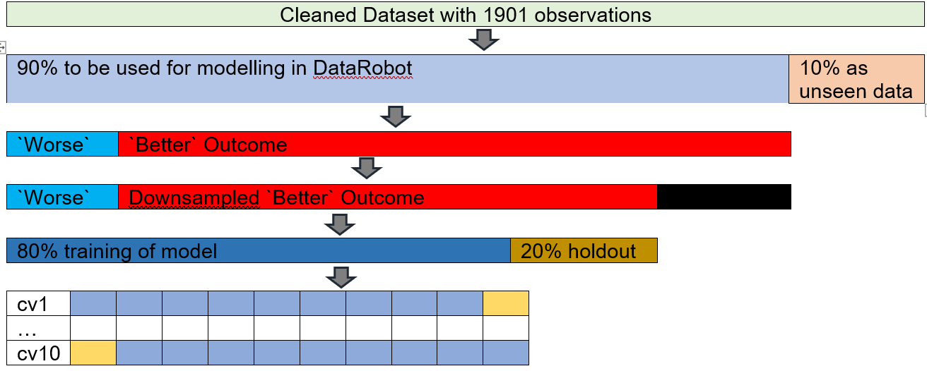
The number of K-fold was increased from the default 5 to 10 folds. The increase in K-folds helps to reduce biasness and therefore reduces the risk of underfitting. Based on the concept of bias and variance trade off, the decrease of biasness will increase the variance. Nonetheless, the sample size of the training set is large enough (1840 rows) to accommodate this increase in folds without adversely compromising variance. Additionally, 10-fold cross validation is the default number of folds for some modelling programs; for example, R’s modern modelling meta-package, Tidymodels.
DataRobot was also permitted to search for Interactions among the variables. There is support in identifying interactions as the combined effect of two or more variables maybe different than the impact of the individual constituent variables.
Down-sampling was introduced to address the imbalanced dataset (DataRobot only allows down-sampling). The proportion of positive and negative outcome of the binary classification was imbalanced which [could affect model performance as most models work best when the classes are about equal)(https://towardsdatascience.com/methods-for-dealing-with-imbalanced-data-5b761be45a18). There were 6.25 more Better outcomes than Worse outcomes. DataRobot’s Down-sampling was used to reduce the disparity. Under-sampling can help to address imbalance dataset. The number of Better outcomes were reduced by 20%. Post down-sampling, there was 5.22 Better outcomes than Worse outcomes.

Performance Metric

The performance metric for the binary classification was Area Under the Curve (AUC) which is common in the medical literature. In DataRobot, when down-sampling is used, the performance metric AUC becomes a weighted AUC.

1st Quick Mode

The experiment ran on Quick Mode (DataRobot has 3 modelling modes: Autopilot, Quick, Manual. The student version which I used only has Quick and Manual Mode).

DataRobot API

library(datarobot)
library(tidyverse)
theme_set(theme_light())

ConnectToDataRobot(endpoint = "https://app.datarobot.com/api/v2", 
                   token = "API token key")

## [1] "Authentication token saved"

projects_inDR<-data.frame(name=ListProjects()$projectName, ID=ListProjects()$projectId)

project_ID<-projects_inDR %>% filter(name=="Classify CAP") %>% pull(ID)

## # A tibble: 11 x 2
##    name                        ID                      
##    <chr>                       <chr>                   
##  1 Classify CAP                5f54dce5e5e3f924b99408ee
##  2 CAP Experiment 3            5f3678ff735d1f59f99534ed
##  3 CAP Experiment 2            5f33f9899071ae44ded6de84
##  4 CAP Experiment 1            5f269f896c6a7a1cefaff780
##  5 CAP informative ft          5f2694a9d6e13f1dc8ae17d4
##  6 CleanDR OG cv10             5f2655a8d6e13f1c26ae17c7
##  7 CleanDR OG cv5              5f263758ce243f1bfac853eb
##  8 P04_Readmission(1).csv      5f16dd3b99c1372d672bdde4
##  9 P03_Advertising(1).csv      5f0da6861c29b917239402dc
## 10 P02_LendingClubData2(1).csv 5f047ce3c40c123f3487346b
## 11 P01_TitanicData.csv         5efb44cc60882464b616c03b

List_Model3<-ListModels(project_ID) %>% as.data.frame(simple = F) 

List_Model3 %>% select(modelType, expandedModel, featurelistName, `Weighted AUC.crossValidation`) %>% arrange(-`Weighted AUC.crossValidation`)DT::datatable(rownames = F, options = list(searchHighlight = TRUE, paging= T))

1. Advanced Feature Selection (DR Reduced Features)

During the first round of Quick Mode, DataRobot created other Feature Lists including DR Reduced Features. These feature lists contained curated variables consisting of most important features based on Feature Impact scores from models.

Ft_DR<-GetFeaturelist(project_ID, "5f54e0f611a5fc3a03274070") %>% as_tibble()
Ft_DR$description %>% unqiue()

## [1] "The most important features based on Feature Impact scores from a particular model."

3/13 models used DR Reduced Features in the 1st round of Quick Mode.

List_Model3  %>% count(featurelistName)

## # A tibble: 3 x 2
##   featurelistName            n
##   <chr>                  <int>
## 1 DR Reduced Features M8     3
## 2 L1                         9
## 3 Multiple featurelists      1

Originally 70 variables were used for Quick Mode. 33 variables were identified for DR Reduced Features M8 (32 predictors + 1 outcome).

n_distinct(Ft_DR$features)

## [1] 33

2. Advanced Feature Selection (Top 32 Mean Feature Impact Variables)

The number of predictors were kept the same as the number of predictors in DR Reduced Features to see which technique achieved better performance. The steps for identifying these variables were as follows:

1. All the cross-validation scores for all models were enabled on DataRobot GUI (by default, DataRobot calculates the cross-validation score for the top few models based on the 1st cross-validation fold score). The top 80% of the models based on cross validation AUC were selected. These selected models also had to have sufficient sample size of >64%. 9/13 models passed this screener.

Ft_mean_screenModels<-function(ID_of_project){
# Extract models 
models_listdetails<-ListModels(ID_of_project)
#extract models (df format)
models_df<-as.data.frame(models_listdetails, simple = F)
## top 80%  cv AUC
top80AUC<-quantile(models_df$`Weighted AUC.crossValidation`, probs = seq(0,1,.1), na.rm = T)[["20%"]]
# remove small sample size % models
models_listdetails_big <- Filter(function(m) m$metrics$`Weighted AUC`$crossValidation>top80AUC & m$samplePct >= 64 , models_listdetails)
}

Ft_mean_screened<-Ft_mean_screenModels(project_ID)

as.data.frame(Ft_mean_screened, simple = F) %>% select(expandedModel, featurelistName, `Weighted AUC.crossValidation`) %>% arrange(-`Weighted AUC.crossValidation`) DT::datatable(rownames = F, options = list(searchHighlight = TRUE, paging= T))

2. The unnormalized feature impact score for all the variables in these models were averaged out. Variables in the top 32 mean feature impact score were used to create a new set of Feature List.

Ft_mean_var<-function(Ft_mean_screened_results, ID_of_project){
# feature impact of selected models 
all_impact<- NULL
for(i in 1:length(Ft_mean_screened_results)) {  
     featureImpact <- GetFeatureImpact(Ft_mean_screened_results[[i]])
    featureImpact$modelname <- Ft_mean_screened_results[[i]]$modelType
    all_impact <- rbind(all_impact,featureImpact)
  }

#mean impact
mean_impact<-all_impact %>% group_by(featureName) %>% 
    summarise(avg_impact = mean(impactUnnormalized), .groups="drop")

#top X mean feature impact scores 
## number of predictors for DR
no_of_DRft<-ListFeaturelists(ID_of_project) %>% as.data.frame() %>% filter(str_detect(name, "DR Reduced")) %>% nrow()-1 # minus 1 as one of the variables is the target 

##top X mean feature impact scores 
top_mean_names<-mean_impact %>% slice_max(order_by = avg_impact, n=no_of_DRft ) %>% pull(featureName)

# multiple output https://stackoverflow.com/questions/1826519/how-to-assign-from-a-function-which-returns-more-than-one-value
output<-list(all_impact, top_mean_names)
return (output)
}

Ft_mean_varOutput<- Ft_mean_var(Ft_mean_screened, project_ID)

The calculation can be seen on DataRobot’s GUI.

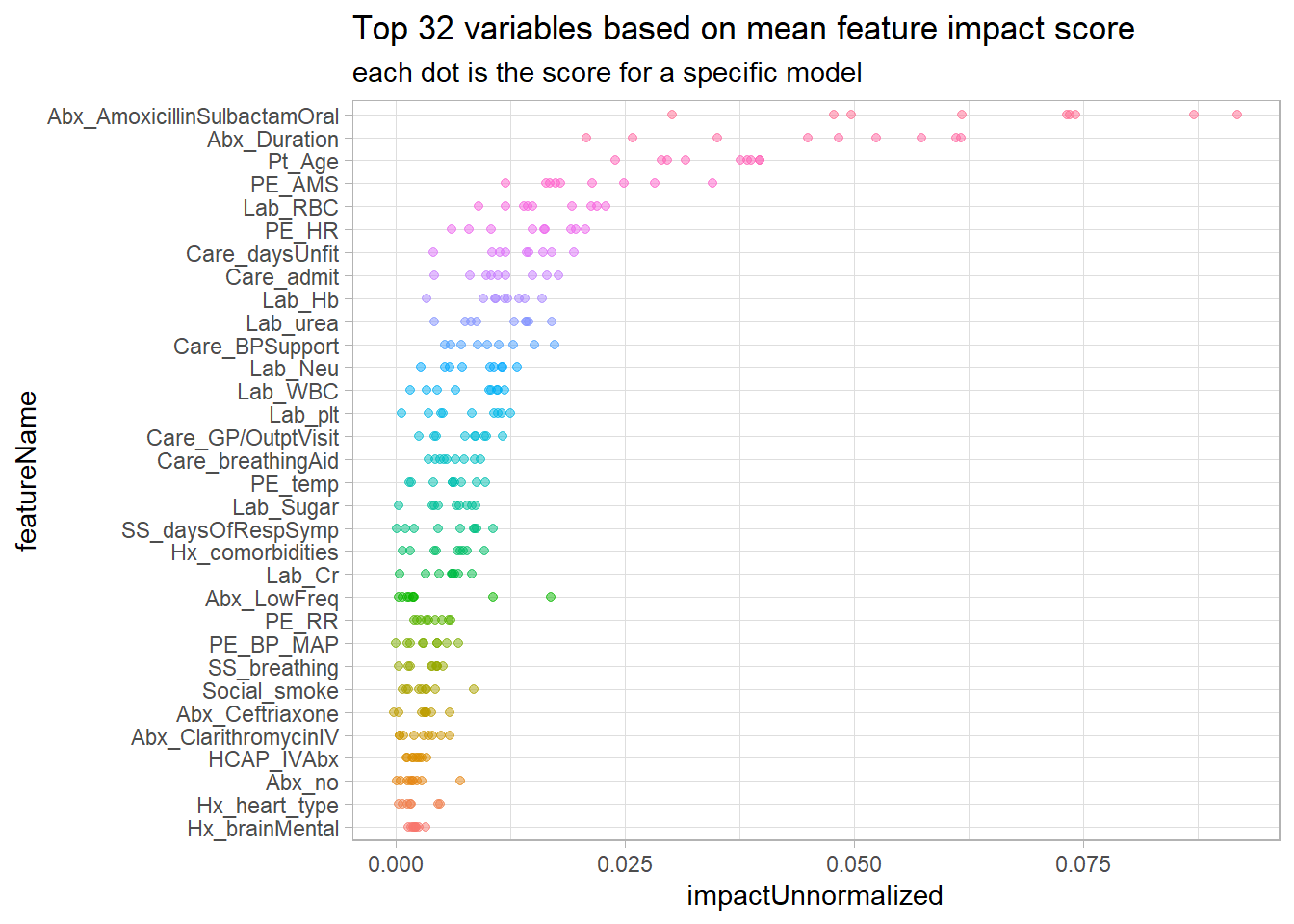
The top 32 variables based on mean feature impact score and their respective feature impact score for each model is plotted here.

Ft_mean_varOutput[[1]]%>%  
  filter(featureName %in% Ft_mean_varOutput[[2]]) %>% 
  mutate(featureName= fct_reorder(featureName, impactUnnormalized, .fun =mean)) %>%
     ggplot(aes(featureName, impactUnnormalized, colour=featureName))+ geom_point(alpha=.5) + coord_flip() + theme(legend.position="none") + labs(title = "Top 32 variables based on mean feature impact score", subtitle = "each dot is the score for a specific model")

New Feature List using the top 32 mean feature impact variables was created.

Feature_id_percent_rank = CreateFeaturelist(project_ID, 
                                            listName= "mean ft impact" , 
                                            featureNames= 
  Ft_mean_varOutput[[2]][1:length(Ft_mean_varOutput[[2]])])$featurelistId

## [1] "Featurelist mean ft impact created"

DR Features vs Top 32 mean Feature Impact variables

Both Feature Lists had these predictors in common

intersect(Ft_mean_varOutput[[2]], Ft_DR$features)

##  [1] "Abx_AmoxicillinSulbactamOral" "Abx_Duration"                
##  [3] "Pt_Age"                       "PE_AMS"                      
##  [5] "Lab_RBC"                      "PE_HR"                       
##  [7] "Care_daysUnfit"               "Care_admit"                  
##  [9] "Lab_Hb"                       "Lab_urea"                    
## [11] "Care_BPSupport"               "Lab_Neu"                     
## [13] "Lab_WBC"                      "Lab_plt"                     
## [15] "Care_GP/OutptVisit"           "Care_breathingAid"           
## [17] "PE_temp"                      "Lab_Sugar"                   
## [19] "SS_daysOfRespSymp"            "Hx_comorbidities"            
## [21] "Lab_Cr"                       "Abx_LowFreq"                 
## [23] "PE_RR"                        "PE_BP_MAP"                   
## [25] "SS_breathing"                 "Social_smoke"                
## [27] "Abx_Ceftriaxone"              "Abx_ClarithromycinIV"        
## [29] "HCAP_IVAbx"                   "Abx_no"                      
## [31] "Hx_brainMental"

The only difference was that the top 32 mean Feature Impact variables contained medical history on the type of heart disease the patient had.

setdiff(Ft_mean_varOutput[[2]], Ft_DR$features)

## [1] "Hx_heart_type"

Running 2nd Quick Mode

Another round of Quick Mode was ran with both of the new Feature Lists created with advanced feature selection. Again, cross validation scores for all models was calculated. 8 additional models were generated with DR Reduced features (the other 3 was previously generated in the 1st round of Quick Mode). 10 additional models were generated with the Top 32 mean Feature Impact score variables.

#Get all the models from 1st and 2nd Quick Mode 
List_Model322<-ListModels(project_ID) %>% as.data.frame(simple = F) 

List_Model322 %>% count(featurelistName)

## # A tibble: 4 x 2
##   featurelistName            n
##   <chr>                  <int>
## 1 DR Reduced Features M8    11
## 2 L1                         9
## 3 mean ft impact            10
## 4 Multiple featurelists      1

In the next post, the results from all the models from both runs of Quick Mode will be analysed.