Predicting pneumonia outcomes: Results (using DataRobot API)
This post is a supplementary material for an assignment. The assignment is part of the Augmented Machine Learning unit for a Specialised Diploma in Data Science for Business. The aim of this project is to classify if patients with Community Acquired Pneumonia (CAP) became better after seeing a doctor or became worse despite seeing a doctor.
Previously, EDA (part1, part 2)and feature enginnering was done in R. The dataset was then imported into DataRobot for the first round of basic modelling (the aim of the assignment was to use DataRobot). Next, R was used for advanced feature selection in the second round of DataRobot’s modelling. The post here will outline the results after both rounds of modelling.
All models
library(datarobot)
library(tidyverse)
theme_set(theme_light())
ConnectToDataRobot(endpoint = "https://app.datarobot.com/api/v2",
token = "API token key")## [1] "Authentication token saved"# Saving the relevant project ID
projects_inDR<-data.frame(name=ListProjects()$projectName, ID=ListProjects()$projectId)
project_ID<-projects_inDR %>% filter(name=="Classify CAP") %>% pull(ID)After 2 runs of modelling (basic and with advanced feature selection), a total of 31 models was created.
# Saving the models
List_Model3<-ListModels(project_ID) %>% as.data.frame(simple = F)

List_Model3 %>% select(expandedModel, featurelistName, `Weighted AUC.crossValidation`) %>% arrange(-`Weighted AUC.crossValidation`) %>% DT::datatable(rownames = F, options = list(searchHighlight = TRUE, paging= T))
TPR and TNR
3 metrics were used to compare the models, namely, AUC, sensitivity/ true positive rate (TPR) and specificity/ true negative rate (TNR). AUC was the primary metric. TPR and TNR had to be extracted separately. DataRobot determines the TPR and TNR based on the maximized F1 score (though the TPR and TNR can be adjusted based on other F1 score). There is an indirect way and direct way to extract the TPR and TNR .
1. Indirect
The TPR and TNR can be indirectly calculated by using the values in the confusion matrix.
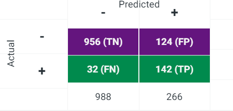
# extract all modelId
model_id<-List_Model3 %>% filter(!is.na(`Weighted AUC.crossValidation`)) %>% pull(modelId)
However, the API was unable to obtain the confusion matrix.
(GetModel(project_ID, model_id[1]) %>% GetConfusionChart(source = DataPartition$VALIDATION))

(GetModel(project_ID, model_id[1]) %>% GetConfusionChart(source = DataPartition$CROSSVALIDATION))

(GetModel(project_ID, model_id[9]) %>% GetConfusionChart(source = DataPartition$VALIDATION))

(GetModel(project_ID, model_id[9]) %>% GetConfusionChart(source = DataPartition$CROSSVALIDATION))
## [1] "Error: (404) No confusion chart for validation"## [1] "Error: (404) No confusion chart for validation"## [1] "Error: (404) No confusion chart for validation"## [1] "Error: (404) No confusion chart for validation"2. Direct way
The TPR and TNR is directly printed on the Selection Summary under the ROC option in the DataRobot GUI.

The same can be accessed via the GetRocCurve function in the API.
# loop to get all TNR and TPR from ROC Curve option. https://stackoverflow.com/questions/29402528/append-data-frames-together-in-a-for-loop
TPR_TNR<-data.frame()

for (i in model_id){
selection_summary<-GetModel(project_ID, i) %>% GetRocCurve(source = DataPartition$CROSSVALIDATION)

temp<-selection_summary$rocPoints%>%
  filter(f1Score==max(f1Score)) %>% select(truePositiveRate, trueNegativeRate) %>%
  mutate(modelId= i)

TPR_TNR<-bind_rows(TPR_TNR, temp)
}

TPR_TNR %>% head()
## # A tibble: 6 x 3
## truePositiveRate trueNegativeRate modelId
## <dbl> <dbl> <chr>
## 1 0.724 0.903 5f564d6cdf91a0559ffbfb8c
## 2 0.621 0.931 5f54de5d269d39249ea468a3
## 3 0.770 0.876 5f54de5d269d39249ea468a2
## 4 0.649 0.936 5f54de5d269d39249ea468a4
## 5 0.787 0.886 5f54de5d269d39249ea468a7
## 6 0.736 0.906 5f564d880a859d0d17d859c8Updating main dataframe
TPR_TNR was joined with the main dataframe, List_Model3, to allow all metrics to be in a common dataframe.
List_Model3<-List_Model3 %>% left_join(TPR_TNR, by = "modelId") %>%
  # select columns of interest
  select(modelType, expandedModel, modelId, blueprintId, featurelistName, featurelistId, `Weighted AUC.crossValidation`, TPR=truePositiveRate, TNR=trueNegativeRate) %>% mutate(`Weighted AUC.crossValidation`= as.double(`Weighted AUC.crossValidation`))
## Warning in mask$eval_all_mutate(dots[[i]]): NAs introduced by coercionResults
Performance of models
The AUC was high and similar for all models. For this study, it was more important to identify as many patients who became worse despite seeing a doctor (i.e. true positive). Identification of these patients with poor outcomes would allow better intervention to be provided to increase their chances of a better clinical evolution. Thus, models with high TPR were preferred. Though there is a trade-off between TPR and TNR, selecting models with higher TPR in this study would not compromise TNR drastically as TNR were high and similar for all models. TNR was better in TPR for all models due to the imbalanced dataset. The models saw more negative classes during training and thus were more familiar to identify negative cases during validation/testing.
List_Model3 %>% pivot_longer(cols = c(`Weighted AUC.crossValidation`, TPR, TNR), names_to="metric") %>% ggplot(aes(metric, value, fill=metric)) + geom_boxplot(alpha=.5) ## Warning: Removed 3 rows containing non-finite values (stat_boxplot).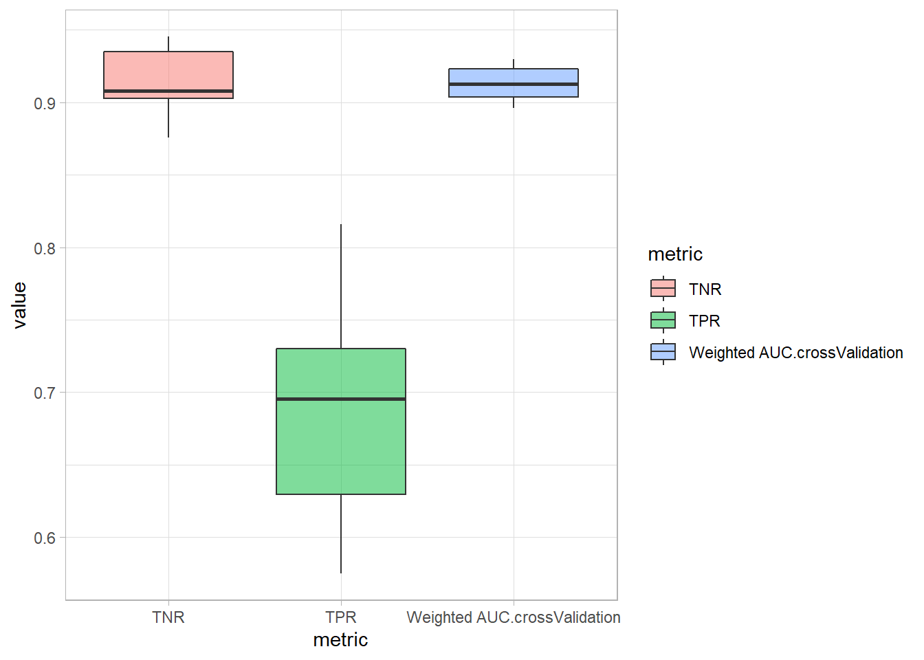
Performance of Advanced Feature Selection
Between models generated using advanced feature selection, the AUC was high for both DR Reduced Features and the top 32 mean feature impact variables. There was less variability for DR Reduced Features. DR Reduced Features had higher average TPR but larger variation compared to the top 32 mean feature impact variables. A model using DR Reduced Features had the highest TPR.
List_Model3 %>% pivot_longer(cols = c(`Weighted AUC.crossValidation`, TPR, TNR), names_to="metric") %>% ggplot(aes(metric, value, fill=featurelistName)) + geom_boxplot(alpha=.5) ## Warning: Removed 3 rows containing non-finite values (stat_boxplot).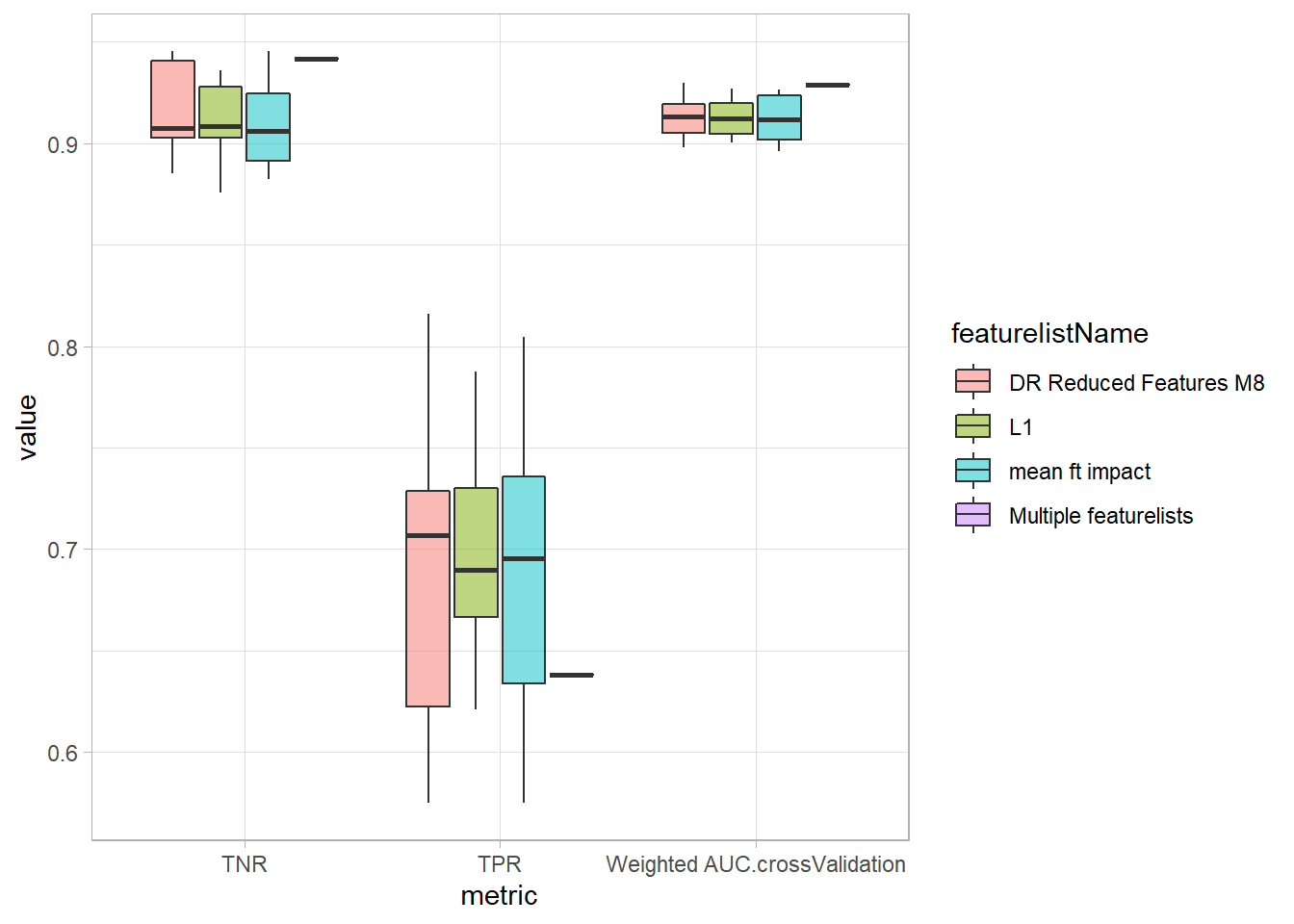
Selecting a model for deployment
Out of the 31 models, a handful of the models were selected to be compared against the holdout set to determine the most appropriate model for deployment. The models had to have high AUC and high TPR (as shared above TPR is prioritise over TNR).
deploy_all<-List_Model3 %>% mutate(
  AUC_rank=min_rank(desc(`Weighted AUC.crossValidation`)),
  TPR_rank= min_rank(desc(TPR)), #min rank will have same ranking for ties
         TNR_rank= min_rank(desc(TNR))) %>% select(modelType, featurelistName, `Weighted AUC.crossValidation`, AUC_rank, TPR, TPR_rank, TNR, TNR_rank, modelId, blueprintId) %>%
  mutate(across(.cols = c(`Weighted AUC.crossValidation`, TPR, TNR),
                .fns = ~round(.x, 5)))

deploy_all %>% select(-c(modelId, blueprintId))
## # A tibble: 31 x 8
## modelType featurelistName `Weighted AUC.c~ AUC_rank TPR TPR_rank TNR
## <chr> <chr> <dbl> <int> <dbl> <int> <dbl>
## 1 eXtreme ~ DR Reduced Fea~ NA NA NA NA NA
## 2 Keras Sl~ DR Reduced Fea~ 0.909 19 0.724 11 0.903
## 3 RuleFit ~ L1 0.905 21 0.621 24 0.931
## 4 Keras Sl~ L1 0.908 20 0.770 4 0.876
## 5 eXtreme ~ L1 0.927 4 0.649 21 0.936
## 6 RandomFo~ L1 0.919 12 0.787 3 0.886
## 7 Generali~ mean ft impact 0.923 8 0.736 6 0.906
## 8 Generali~ L1 0.920 11 0.724 11 0.903
## 9 AVG Blen~ Multiple featu~ 0.929 2 0.638 22 0.942
## 10 RandomFo~ mean ft impact 0.914 15 0.695 15 0.913
## # ... with 21 more rows, and 1 more variable: TNR_rank <int>The 5 models were:
- The model with the highest AUC which also had the highest TPR
- The model with the 2nd highest AUC
- The model with the 2nd highest TPR
- A model with a relatively balanced high AUC and TPR (7th for AUC and 4th for TPR)
- Another model with a relatively balanced high AUC and TPR (5th for AUC and 6th for TPR)
(deploy_all %>% select(-c(modelId, blueprintId)) %>% filter(AUC_rank %in% c(1,2,7,5)| TPR_rank==2)) %>% DT::datatable(rownames = F, options = list(searchHighlight = TRUE, paging= T))# model ID for the 5 candidates
deploy_modelsId<-deploy_all %>% filter(AUC_rank %in% c(1,2,7,5)| TPR_rank==2) %>% pull(modelId)The holdout dataset was unlocked and the performance of these 5 models on the holdout set was compared.
# extract model and holdout AUC
deploy_models<-ListModels(project_ID) %>% as.data.frame(simple = F)

deploy_models<-deploy_models%>%  select(modelType, expandedModel, featurelistName, `Weighted AUC.holdout`, modelId, blueprintId) %>% filter(modelId %in% deploy_modelsId)

# extract holdout TPR and TNR
TPR_TNR_holdout<-data.frame()

for (i in deploy_modelsId){
selection_summary<-GetModel(project_ID, i) %>% GetRocCurve(source = DataPartition$HOLDOUT)

temp<-selection_summary$rocPoints%>%
  filter(f1Score==max(f1Score)) %>% select(truePositiveRate, trueNegativeRate) %>%
  mutate(modelId= i)

TPR_TNR_holdout<-bind_rows(TPR_TNR_holdout, temp)
}

# join all metrics
deploy_results<- left_join(deploy_models, TPR_TNR_holdout, by="modelId") %>% distinct(modelId, .keep_all = T) %>% rename(TPR= truePositiveRate, TNR=trueNegativeRate)
Based on the holdout metrics, Light Gradient Boosted Trees with early stopping (Light GBT) was selected as the model for deployment. Although Light GBT did not have the highest holdout AUC, its AUC of 0.94033 was still close the maximum AUC of 0.95695. The merits of Light GBT was its high TPR and TNR and it had the smallest difference between TPR and TNR. Moreover, it had the highest TPR which is valued for this classification problem.
# plot
(deploy_results %>% unite("model", c(modelType, featurelistName), sep=":") %>% pivot_longer(cols = c(`Weighted AUC.holdout`, TPR, TNR), names_to="metric") %>% ggplot(aes(model, value, colour=metric)) + geom_point(alpha=.7) + coord_flip()+ labs(x="", title = "Metrics of Potential Models for Deployment", subtitle = "tested on holdout set")+
  scale_x_discrete(labels = scales::wrap_format(55))) #https://stackoverflow.com/questions/21878974/auto-wrapping-of-labels-via-labeller-label-wrap-in-ggplot2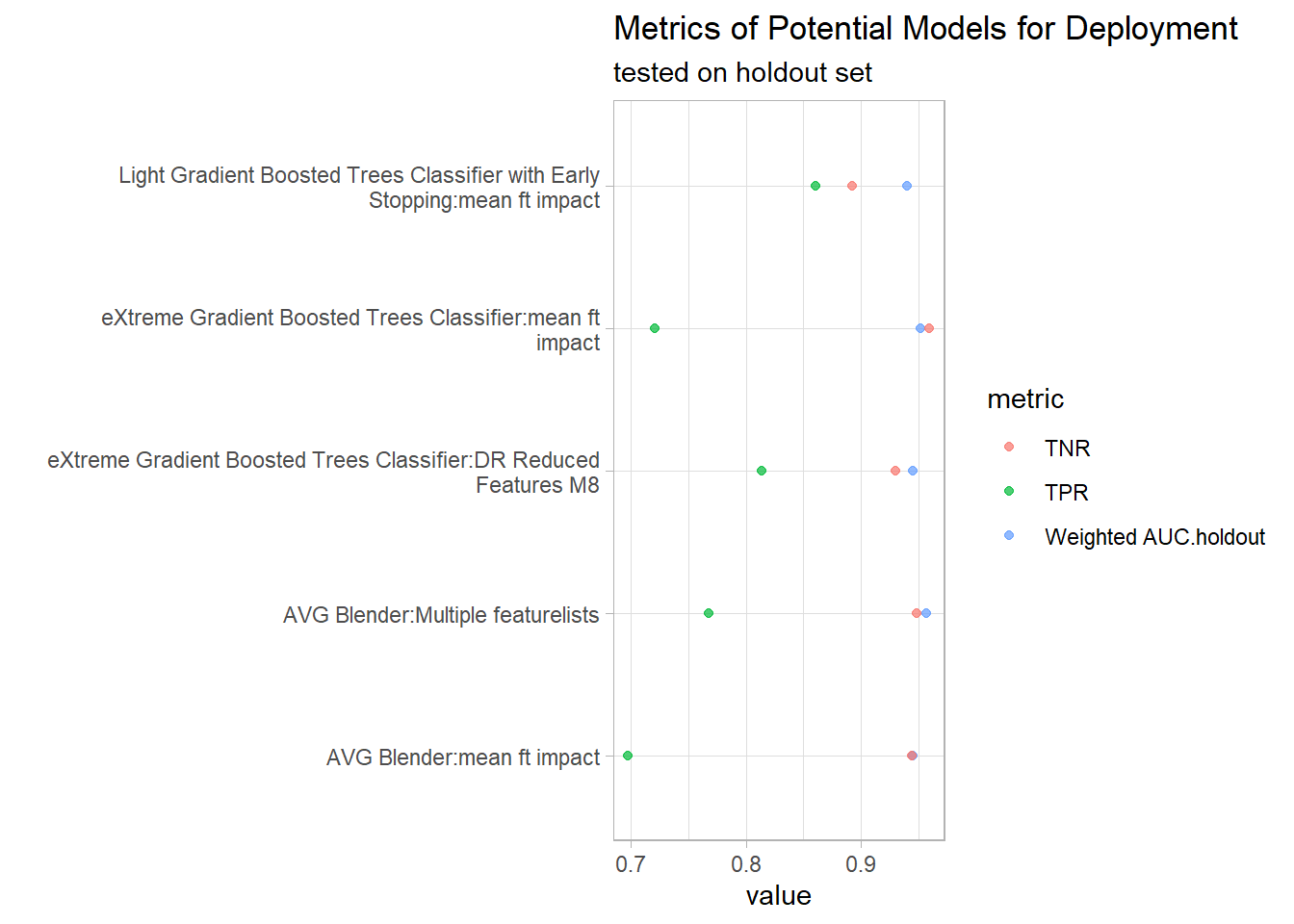
LightGBT
Description of the deployed Light GBT
# modelId of Light GBT
LightGBT_Id <-deploy_results %>% filter(str_detect(modelType, "Light")) %>% pull(modelId)
#blueprint
LightGBT_blueprint<-GetModelBlueprintDocumentation(project_ID, LightGBT_Id) %>% data.frame()
(glue::glue ("Description of the deployed model:: \n{LightGBT_blueprint$description}"))## Description of the deployed model::
## The Classifier uses the LightGBM implementation of Gradient Boosted Trees.
## LightGBM is a gradient boosting framework designed to be distributed and efficient with the following advantages:
## Gradient Boosting Machines (or Gradient Boosted Trees, depending on who you ask to explain the acronym ‘GBM’) are a cutting-edge algorithm for fitting extremely accurate predictive models. GBMs have won a number of recent predictive modeling competitions and are considered among many Data Scientists to be the most versatile and useful predictive modeling algorithm. GBMs require very little preprocessing, elegantly handle missing data, strike a good balance between bias and variance and are typically able to find complicated interaction terms, which makes them a useful “swiss army knife” of predictive models. GBMs are a generalization of Freund and Schapire’s adaboost algorithm (1995) to handle arbitrary loss functions. They are very similar in concept to random forests, in that they fit individual decision trees to random re-samples of the input data, where each tree sees a boostrap sample of the rows of a the dataset and N arbitrarily chosen columns where N is a configural parameter of the model. GBMs differ from random forests in a single major aspect: rather than fitting the trees in parallel, the GBM fits each successive tree to the residual errors from all the previous trees combined. This is advantageous, as the model focuses each iteration on the examples that are most difficult to predict (and therefore most useful to get correct). Due to their iterative nature, GBMs are almost guaranteed to overfit the training data, given enough iterations. The 2 critial parameters of the algorithm; therefore, are the learning rate (or how fast the model fits the data) and the number of trees the model is allowed to fit. It is critical to cross-validate one of these 2 parameters.
## Early stopping is used to determine the best number of trees where overfitting begins. In this manner GBMs are usually capable of squeezing every last bit of information out of the training set and producing the model with the highest possible accuracy.Hyper-parameters which were tuned::
### tuned values
# list within a list
para<-GetModel(project_ID, LightGBT_Id) %>% GetTuningParameters()

# option 1 to covert to df
para_df<-summary(para)

# option 2 to convert to df2
#paraName<- list()
#value<-list()

#for(i in 1:18){
#  paraName_temp<-para[["tuningParameters"]][[i]][["parameterName"]] %>% data.frame()
#  paraName[[i]]<-paraName_temp

#  value_temp<-para[["tuningParameters"]][[i]][["currentValue"]] %>% data.frame()
#  value[[i]]<-value_temp
#}

#paraName<-bind_rows(paraName)

#value_df<-data.frame()
#for (i in 1:length(value)){
#  temp<- value[[i]] %>% data.frame()
#  value_df<-rbind(temp, value_df)
#}

#bind_cols(paraName, value_df)
### parameters description
para_describe<-LightGBT_blueprint %>%
# as num ID to para w no ID (e.g. parameters.type-> parameters.type.0)
rename_with(.fn=~paste0(.x, ".0") , .cols=matches("parameter(.*)[^0-9]$")) %>%
# select only parameters var
select(starts_with("parameter")) %>%
# parameters.type.0-> type.0
rename_with(.fn=~str_replace(.x, "parameters.", "")) %>%
# type.0-> type_parameter0.
##need [] to encapsulate full stop, list of permitted char
rename_with(.fn=~str_replace(.x, "[.]", "_parameter")) %>%
# https://tidyr.tidyverse.org/articles/pivot.html#multiple-observations-per-row-1
pivot_longer(cols=everything(), names_to = c(".value", "parameter"), names_sep = "_") %>%
# parameter10-> 10
## sep the alphabets not numbers, convert to int
separate(parameter, into = c(NA, "para"), sep = "[a-z]+", convert = T) %>%
# remove parthesis and abbreviation for name
mutate(name= str_remove(name, "\\(.*\\)") %>% str_trim()) There is an extra tuned parameter in para_df which is the type of classification. This extra parameter was ignored.
anti_join(para_df, para_describe, by="name") ## # A tibble: 1 x 4
## name current default constraint
## <chr> <chr> <chr> <chr>
## 1 objective binary binary select from: binary, multiclass, multiclassovaDescription of the hyper-parameters and the tuned values
left_join(para_describe, para_df, by="name") %>% select(parameter=name, description, limits=constraint, default_value=default, tuned_values=current) %>% DT::datatable(rownames = F, options = list(searchHighlight = TRUE, paging= T))Reviewing deployed model
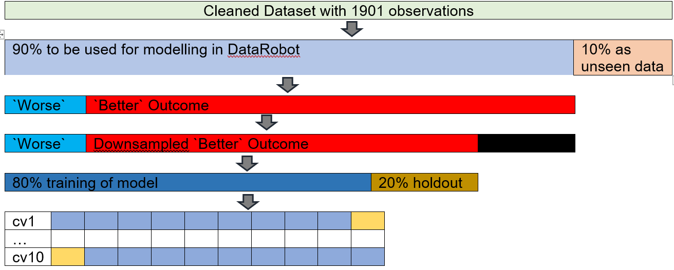
Light GBT was deployed and used to make predictions on unseen data. An unseen dataset was reserved earlier to evaluate the deployed model’s performance in the real world.
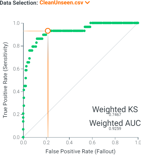
The AUC was 0.926 for the unseen data which is close to the AUC for the holdout set (0.94) suggesting Light GBT is neither overfitting nor underfitting the unseen data.
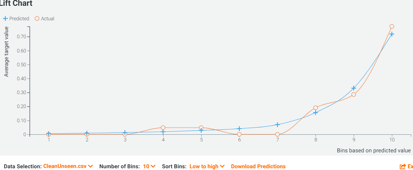
The frequent interlacing of the Predicted and the Actual Lines in the Lift Chart also accentuated that the Light GBT is neither underestimating nor overestimating.
The sensitivity of 0.759 was not as high compared to the sensitivity of 0.861 when predicting the holdout set. The smaller sensitivity is likely due to the low absolute number of positive cases in the unseen data. Inspecting purely by numbers, identifying 22/29 positive cases appears rather impressive. However, when the relative proportion was calculated, it appeared less remarkable.

Adopting ML (is better than not adopting ML)
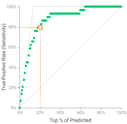
The powerful predictive properties of machine learning can determine patients with CAP who will deteriorate despite receiving medical treatment. According to the cumulative lift chart, when Light GBT was used to predict the unseen data, the top 20% predictions based on the model’s probability of worse CAP outcomes contained almost 4 times more cases compared to no modelling.
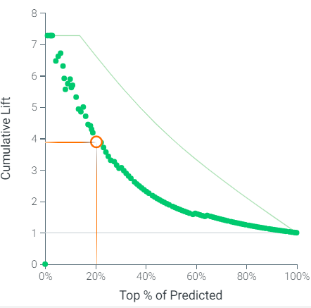
A CAP watch list targeting 20% of the patients based on Light GBT can expect to have almost 4 times more patients with poorer outcomes compared to not using a model and selecting a random sample of patients. Doctors can pay closer attention to these patients who are on the watch list as they are almost 4 times more likely to have worse clinical evolution.
According to the cumulative gain chart, the CAP watch list can expect to have almost 80% of the patients with worse outcomes using the top 20% predictions based on Light GBT.
Thoughts on DataRobot
Automated machine learning (AutoML) platforms like DataRobot reduces the amount of manual input in a data science project and democratizes data science to less data literate clinicians. Nonetheless, there are pitfalls to AutoML as manual review is still required to enhance the models and validate that the variables driving the predictions make clinical sense. As seen in this series, an augmented machine learning approach integrating domain knowledge and the context of data when using AutoML platforms will be more appropriate, especially in healthcare where human life is at stake.
For functions which are available in both DataRobot GUI and via R API, the ease of using the mouse makes it more convenient to use the GUI. However, without documentation of code, the project will be harder to reproduce. The option of using either GUI or via the API may create confusion among the team on which steps to be done in the GUI or via the API. Additionally, there are functions which are not available via the API. While there is a function via the API to predict on the unseen dataset, there is no function to provide the performance on the unseen dataset. Thus, the above cumulative lifts and gain charts were screen shots.
Future work
- Deploying the model. However, deployment is not an option with the student’s version of
DataRobot. - Visualizing
DataRobot’s results inTableau. However, this requires the deployment option. - Running customized models in
DataRobot. However, model registry is required but is not an option with the student’s version ofDataRobot. - Modelling the entire project in either
R’stidymodelsorpython’ssklearn.